Antenna Input Impedance Explained

Input resistance and reactance of a 146 MHz dipole against frequency: resistance rising slowly through about 72 ohms, reactance crossing zero at 146 MHz with a positive slope — Input impedance of a 146 MHz half-wave dipole from 120 to 170 MHz (Method of Moments). The reactance (purple) crosses zero at resonance with a positive slope, like a series RLC circuit; the resistance (blue) is 71.9 Ω there and rises slowly with frequency. Try it in the Dipole & Monopole Antenna Calculator →

Introduction to Antenna Input Impedance

An antenna connects to a transmitter or receiver through two terminals. Whatever happens beyond them — radiation, heating, energy stored in the near field — the circuit only sees a voltage V_A and a current I_A at a given frequency. Their ratio is the input impedance, which IEEE 145 defines as "the impedance presented by an antenna at its terminals."

Input impedance decides how much of the available power actually enters the antenna (Part 8), how efficiently that power is radiated (Part 9), and over what bandwidth the antenna can be used (Part 10). It is the single most-measured antenna property, and the first thing a designer tunes.

Definition of Input Impedance

Draw a closed surface around the antenna that crosses the feed at the terminals and extends to the far field. Applying the complex Poynting theorem (Part 5) to the volume inside, the complex power delivered at the terminals splits into three parts:

Input impedance from the complex power balance

\frac{1}{2} V_{A} I_{A}^{*} = P_{rad} + P_{loss} + 2 j ω (W_{m} - W_{e})

Z_{A} = \frac{V_{A}}{I_{A}} = \frac{P_{rad} + P_{loss} + 2 j ω (W_{m} - W_{e})}{\frac{1}{2} {| I_{A} |}^{2}} = R_{r} + R_{L} + j X_{A}

Multiplying numerator and denominator by I_A gives the second form. W_m and W_e are the time-average magnetic and electric energies stored around the antenna (mostly in the reactive near field, Part 3). Each part of the impedance has a direct physical meaning.

Resistance and Reactance Components

Component	Defined by	Physical meaning	Typical values
Radiation resistance R_r	P_rad = ½\|I_A\|²R_r	Power that leaves as radiation	0.01 Ω (tiny loop) to ≈ 300 Ω (folded dipole)
Loss resistance R_L	P_loss = ½\|I_A\|²R_L	Heat in conductors, dielectrics and nearby ground	mΩ (thick copper) to tens of Ω (thin steel, poor ground)
Reactance X_A	X_A = 2ω(W_m − W_e)/(½\|I_A\|²)	Net stored energy: inductive if magnetic energy dominates, capacitive if electric dominates	−2000 Ω (short dipole) to +500 Ω (long dipole)

Only R_r is useful. R_L wastes power, and X_A, although it consumes no power, prevents power from being delivered unless it is cancelled by a matching network.

Radiation Resistance

Radiation resistance is the fictitious resistance that would dissipate the radiated power if it carried the antenna current. It must always be referred to a specific current — usually the feed current, sometimes the current maximum. For the Hertzian dipole (Part 1) it is 80π²(L/λ)². For the half-wave dipole we integrate the far-field power:

Radiation resistance of a half-wave dipole — derivation

P_{rad} = \frac{η I_{0}^{2}}{8 π^{2}} 2 π \int_{0}^{π} \frac{\cos^{2} (\frac{π}{2} \cos θ)}{\sin θ} d θ = \frac{η I_{0}^{2}}{8 π} Cin (2 π)

R_{r} = \frac{2 P_{rad}}{I_{0}^{2}} = \frac{η}{4 π} Cin (2 π) = 30 \times 2.4377 = 73.1 Ω

The θ-integral is evaluated with the substitution x = cos θ and partial fractions; it equals ½Cin(2π), where Cin(x) = ∫₀ˣ (1 − cos t)/t dt = 2.4377 for x = 2π. Because the half-wave dipole's current maximum is at the feed, 73.1 Ω is also its input radiation resistance.

Referring R_r to the feed

For a dipole of any length L with the sinusoidal current I(z) = I_m sin[k(L/2 − |z|)], the radiated power is fixed, but the feed current is I_m sin(kL/2). Since ½I_m²R_m = ½|I_feed|²R_in:

Radiation resistance at the feed

R_{in} = \frac{R_{m}}{\sin^{2} (k L / 2)}

R_m is the radiation resistance referred to the current maximum. For L = λ the feed is at a current null and R_in becomes very large (several thousand ohms in practice, limited by the departure of the real current from a pure sine).

Loss Resistance

At radio frequencies, current flows in a thin skin at the conductor surface. The current density decays as e^(−d/δ) into the metal, where δ is the skin depth:

Skin depth and surface resistance

δ = \frac{1}{\sqrt{π f μ σ}} R_{s} = \frac{1}{σ δ} = \sqrt{\frac{π f μ}{σ}} Ω per square

For copper (σ = 5.8 × 10⁷ S/m) δ = 66 µm/√(f in MHz): 5.5 µm at 146 MHz, 1.3 µm at 2.45 GHz. Surface roughness and plating thinner than a few δ increase the effective R_s.

A round wire of radius a ≫ δ behaves like a strip of width 2πa with resistance R_s per square. A short length dz carrying current I(z) dissipates ½|I(z)|²R_s dz/(2πa). Integrating along a half-wave dipole with sinusoidal current and referring to the feed current I₀:

Loss resistance of a half-wave dipole — derivation

P_{loss} = \frac{R_{s}}{2 π a} \int_{- L / 2}^{L / 2} \frac{1}{2} I_{0}^{2} \cos^{2} (k z) d z = \frac{1}{2} I_{0}^{2} \frac{L R_{s}}{4 π a} \Rightarrow R_{L} = \frac{L R_{s}}{4 π a}

The average of cos² over a half-cycle is ½, which halves the result compared with a uniform current (L R_s/2πa). For a short dipole with a triangular current the average of the square is ⅓, giving L R_s/(6πa).

Other loss mechanisms add their own resistances in series: dielectric loss in substrates and radomes (dominant in printed antennas, Part 9), ground loss under monopoles and low dipoles, loss in loading coils and matching components, and current on the outside of a coaxial feed.

Antenna Reactance

Reactance comes from energy stored near the antenna. A short dipole is essentially two small capacitor plates (the arms) far apart: electric energy dominates and X_A is large and negative. A small loop is essentially an inductor: magnetic energy dominates and X_A is positive. As a dipole lengthens towards λ/2, the stored electric and magnetic energies come into balance, and X_A passes through zero.

A transmission-line model

An open-circuited two-wire line of length ℓ has input impedance Z = −jZ₀ cot(kℓ). Treating each arm of a dipole as one conductor of a flared line of length L/2 and average characteristic impedance Z₀ gives a useful approximation:

Transmission-line estimate of dipole reactance

X_{A} \approx - Z_{0} \cot (\frac{k L}{2}) Z_{0} \approx 120 [\ln (\frac{L}{2 a}) - 1] Ω

Correctly predicts a capacitive reactance for L < λ/2, zero near λ/2, an inductive reactance above, and that thicker wires (smaller Z₀) have smaller reactance. For short dipoles it is accurate; near λ/2 it ignores radiation and becomes only qualitative (Example 9).

The induced-EMF method

A more accurate classical result integrates the near field of the assumed sinusoidal current along the wire surface. It yields closed forms in terms of the sine and cosine integrals Si and Ci. For L = λ/2 the result is the textbook impedance:

Input impedance of an infinitely thin half-wave dipole

Z_{in} = \frac{η}{4 π} Cin (2 π) + j \frac{η}{4 π} Si (2 π) = 73.1 + j 42.5 Ω

Si(2π) = 1.4182. A half-wave dipole is slightly inductive; shortening it by 2–5% (more for thicker wires) removes the reactance, and at that resonant length R_in is a little below 73 Ω.

Relationship Between Antenna Length and Input Impedance

Fig 1 — Input resistance and reactance of a centre-fed dipole against length (induced-EMF method). The reactance crosses zero just below λ/2; a thicker wire (a = 0.01 λ, dashed) has a flatter reactance curve and therefore a wider bandwidth

R_in (both radii)X_in, thin wire a = 0.001 λX_in, thick wire a = 0.01 λ

Wire radius a/λ	Resonant length	R_in at resonance (induced EMF)	L/2a
10⁻⁵	0.488 λ	68 Ω	24 400
10⁻⁴	0.485 λ	67 Ω	2 420
10⁻³	0.478 λ	64 Ω	239
10⁻²	0.457 λ	57 Ω	23

The induced-EMF method slightly under-estimates the resonant resistance of real dipoles: a Method of Moments solution of the 146 MHz, 2.05 mm wire dipole (a/λ = 0.0005) gives 0.479 λ and 71.9 Ω, against 0.480 λ and 65 Ω from the induced-EMF formula. The length is predicted very well; the resistance needs a full numerical solution.

Equivalent Circuit of an Antenna

Over a narrow band around its first resonance, a dipole or monopole behaves like a series RLC circuit; around its anti-resonance (L ≈ λ) it behaves like a parallel RLC. Expanding the reactance in a Taylor series about the resonant frequency ω₀, where X(ω₀) = 0:

Series-RLC model near resonance — derivation

Z_{A} (ω) = R + j (ω L_{s} - \frac{1}{ω C_{s}}) \approx R [1 + j 2 Q \frac{ω - ω_{0}}{ω_{0}}] Q = \frac{ω_{0}}{2 R} {\frac{d X}{d ω}}_{ω_{0}}

ω₀ = 1/√(L_sC_s). For a series RLC, dX/dω = 2L_s at resonance, so Q = ω₀L_s/R as usual. The slope of the reactance at resonance therefore measures the stored energy and sets the bandwidth (Part 10). R = R_r + R_L.

Fig 2 — Lumped equivalent circuits: series RLC near the first resonance of a dipole or monopole; parallel RLC near anti-resonance (L ≈ λ) or for a patch fed at its edge

More elaborate equivalent circuits — chains of RLC sections, Foster forms with several resonances — reproduce the impedance over a decade of frequency and are used to design broadband matching networks. Physically, the series model has a capacitive reactance below resonance (too short: electric energy dominates) and an inductive reactance above it.

Resonant Frequency of an Antenna

An antenna is resonant at a frequency where its input reactance is zero. Resonance does not by itself mean a good match: a resonant half-wave dipole (≈ 70 Ω) gives VSWR 1.4 on a 50 Ω line, and a resonant monopole on a small ground plane may present 20 Ω. Nor is resonance required for radiation: a non-resonant antenna radiates perfectly well once a matching network cancels its reactance. Resonance is valuable because the impedance there is purely resistive and changes slowly, which makes matching easy.

Antenna	First resonance	Z_in at resonance	Next resonance
Thin centre-fed dipole	L ≈ 0.47–0.49 λ	65–72 Ω (series)	L ≈ 0.9–0.95 λ, 1–5 kΩ (parallel)
Monopole on large ground	h ≈ 0.24 λ	32–36 Ω	h ≈ 0.45 λ, high impedance
Folded dipole	L ≈ 0.47 λ	≈ 280–300 Ω	—
Rectangular patch (edge)	L ≈ λ/(2√ε_eff) − 2ΔL	150–400 Ω (inset-feed to 50 Ω)	Higher-order cavity modes
Small loop with tuning capacitor	Set by the capacitor	Very small R; transformer-coupled	—

Input Impedance of a Dipole Antenna

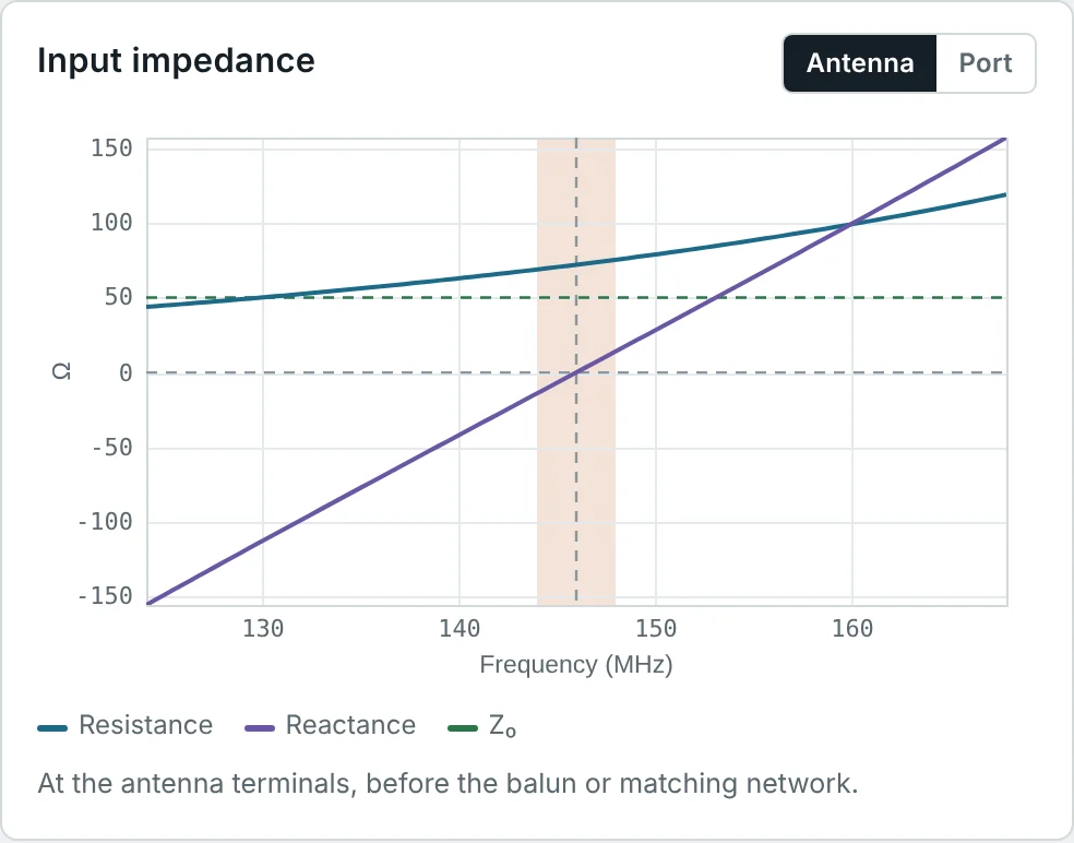
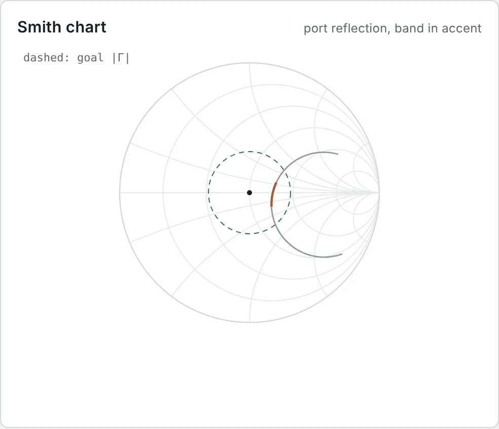
The calculator screenshots show the full frequency response of the 146 MHz dipole. On the Smith chart (Smith Chart & Impedance Matching series) the impedance traces a clockwise arc that crosses the real axis at resonance; the arc is short because a dipole of moderate thickness has a modest Q (Example 7).

Smith chart of the dipole input impedance across 120 to 170 megahertz: a short clockwise arc crossing the real axis near 72 ohms — The same dipole on a Smith chart: a short clockwise arc crossing the real axis at 71.9 Ω (resonance). Try it in the Dipole & Monopole Antenna Calculator →

Input resistance and reactance of a quarter-wave monopole against frequency, with dashed curves showing half of the free-space dipole impedance lying on top of them — Quarter-wave monopole on an ideal ground plane: Z_in = 35.9 Ω at 146 MHz. The dashed curves, half the dipole impedance, coincide with it — image theory at work. Try it in the Dipole & Monopole Antenna Calculator →

Input Impedance of a Monopole Antenna

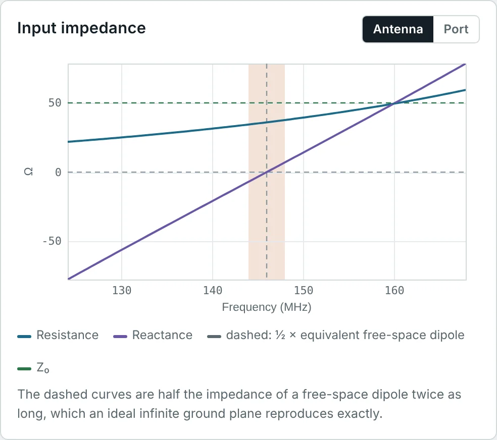
By image theory (Part 2), a monopole of height h on an infinite perfect ground plane produces the same fields above the plane as a dipole of length 2h in free space. It radiates only into the upper half-space, so for the same feed current it radiates half the power, and the feed voltage is half the dipole's (one arm instead of two):

Monopole and dipole impedance

Z_{mono} (h) = \frac{1}{2} Z_{dipole} (L = 2 h) Z_{mono} (λ / 4) = 36.5 + j 21.3 Ω

Valid for a large, highly conducting ground. Small ground planes (vehicle roofs, PCB grounds) raise the impedance and tilt the beam; lossy earth adds ground-loss resistance, which is why broadcast monopoles use 120 buried radials.

Frequency-Dependent Impedance

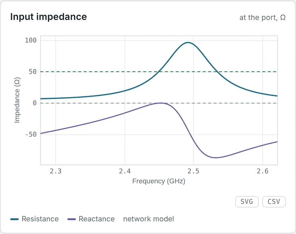
For a fixed antenna, changing frequency changes the electrical length L/λ, so the impedance of Fig 1 is traversed as frequency sweeps. A narrowband antenna (thin dipole, small antenna, patch) has a steep reactance slope and a high Q; a broadband antenna (thick dipole, bowtie, log-periodic, spiral) keeps its impedance nearly constant over a wide range. Comparing the patch and dipole calculator results:

Input resistance and reactance of a 2.45 GHz FR-4 patch antenna against frequency showing a sharp resistance peak and a steep reactance swing — The 2.45 GHz FR-4 patch: a much sharper impedance swing than the dipole (Q ≈ 28 against about 8), which is why patches are narrowband (Part 10). Try it in the Patch Antenna Calculator →

Measuring Antenna Input Impedance

Input impedance is measured with a vector network analyzer (VNA). The VNA measures the complex reflection coefficient S₁₁ at its calibrated reference plane, and the impedance follows from the bilinear transformation of the reflection-coefficient article:

Impedance from a measured S₁₁

Z_{A} = Z_{0} \frac{1 + S_{11}}{1 - S_{11}}

Calibrate at the antenna terminals. SOL (short-open-load) calibration at the end of the cable, or port extension / de-embedding of the feed line, moves the reference plane to the antenna. Otherwise the cable rotates the measured impedance around the Smith chart.
Suppress common-mode current. A balanced antenna fed by coax needs a balun or ferrite choke; otherwise the cable shield becomes part of the antenna and the measurement depends on how the cable is routed.
Mimic the real environment. The reactive near field (Part 3) interacts with nearby objects: measure handset antennas in their housing, ideally with a phantom hand and head.
Use a clear space. Reflections from walls change the impedance of low-directivity antennas slightly; measure in an anechoic chamber or outdoors for accurate values.

Worked Examples

Radiation Resistance of a Half-Wave Dipole

Problem: Evaluate R_r = (η/4π)Cin(2π) with Cin(2π) = 2.4377 and η = 120π Ω. What feed current is needed to radiate 100 W?

R_{r} = 30 \times 2.4377 = 73.1 Ω I_{0} = \sqrt{\frac{2 \times 100}{73.1}} = 1.65 A peak = 1.17 A rms

Answer: R_r = 73.1 Ω; 1.65 A peak (1.17 A RMS)

The feed voltage at resonance would be I₀R ≈ 121 V peak. Short antennas with tiny R_r need very large currents (and develop very large voltages across their reactance) for the same power.

Loss Resistance of a Copper VHF Dipole

Problem: The 146 MHz calculator dipole is 0.985 m of 2.053 mm copper wire (a = 1.027 mm). Find δ, R_s, R_L and the radiation efficiency with R_r = 71.9 Ω.

δ = \frac{1}{\sqrt{π (146 \times 10^{6}) (4 π \times 10^{- 7}) (5.8 \times 10^{7})}} = 5.47 µm R_{s} = 3.15 mΩ

R_{L} = \frac{0.985 \times 0.00315}{4 π \times 0.001027} = 0.24 Ω e_{cd} = \frac{71.9}{71.9 + 0.24} = 99.7 %

Answer: δ = 5.5 µm, R_s = 3.2 mΩ, R_L = 0.24 Ω, efficiency 99.7%

Exactly the 99.7% the calculator reports. Full-size copper dipoles are nearly lossless; losses only matter for thin, poorly conducting or electrically small antennas.

A Stainless-Steel HF Dipole

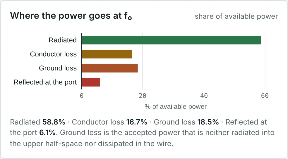
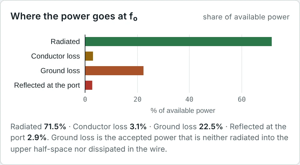
Problem: A 7.15 MHz dipole is 20.6 m of 1.024 mm stainless steel (σ = 1.39 × 10⁶ S/m). Its resonant input resistance over ground is 82.8 Ω. Find R_L and the fraction of the accepted power lost in the wire. Repeat for copper.

R_{s} = \sqrt{\frac{π (7.15 \times 10^{6}) (4 π \times 10^{- 7})}{1.39 \times 10^{6}}} = 4.51 mΩ R_{L} = \frac{20.6 \times 0.00451}{4 π \times 0.000512} = 14.4 Ω

Answer: R_L = 14.4 Ω, about 17% of the accepted power; copper gives 2.2 Ω (3%)

The calculator's power budget shows 16.7% conductor loss for stainless steel and 3.1% for copper, of the available power (Part 9). Stainless steel is 42 times less conductive than copper, so its R_s is √42 = 6.5 times larger.

Power budget bar chart for the stainless steel HF dipole: radiated 58.8 percent, conductor loss 16.7 percent, ground loss 18.5 percent, reflected 6.1 percent — Stainless steel: 16.7% lost in the wire. Try it in the Dipole & Monopole Antenna Calculator →

Power budget bar chart for the copper HF dipole: radiated 71.5 percent, conductor loss 3.1 percent, ground loss 22.5 percent, reflected 2.9 percent — Copper: 3.1% lost in the wire. Try it in the Dipole & Monopole Antenna Calculator →

Short Dipole and Its Loading Coil

Problem: A 1 m dipole of 2 mm wire (a = 1 mm) is used at 30 MHz (L = 0.1 λ). Estimate its input impedance and the series inductance needed to resonate it.

R_{r} = 20 π^{2} {(0.1)}^{2} = 1.97 Ω X_{A} = - 120 (\ln 500 - 1) \cot (18 °) = - 1926 Ω L_{coil} = \frac{1926}{2 π \times 30 \times 10^{6}} = 10.2 µH

Answer: Z_A ≈ 2.0 − j1926 Ω; a 10.2 µH loading coil (the induced-EMF formula gives 2.0 − j1922 Ω)

A coil with Q = 200 has a loss resistance of 1926/200 = 9.6 Ω, five times R_r: the efficiency would be only 17%. This is the practical limit on short, loaded antennas (Part 9).

Quarter-Wave Monopole Impedance

Problem: Use image theory to find the impedance of an exact quarter-wave monopole on a perfect ground, and the resonant impedance of the calculator's 146 MHz monopole if the matching dipole is 71.9 Ω.

Z_{mono} = \frac{73.1 + j 42.5}{2} = 36.5 + j 21.3 Ω \frac{71.9}{2} = 36.0 Ω

Answer: 36.5 + j21.3 Ω exactly at λ/4; about 36 Ω at resonance (calculator: 35.9 Ω)

On 50 Ω coax a resonant monopole gives |Γ| = 0.16, VSWR 1.39 (−15.7 dB return loss). Drooping the radials of a ground-plane antenna downward raises the impedance towards 50 Ω.

Impedance from a Measured S₁₁

Problem: A VNA calibrated at the antenna terminals reads S₁₁ = 0.2∠60° in a 50 Ω system. Find Z_A.

S_{11} = 0.1 + j 0.1732 Z_{A} = 50 \frac{1.1 + j 0.1732}{0.9 - j 0.1732} = 57.1 + j 20.6 Ω

Answer: Z_A = 57.1 + j20.6 Ω (inductive: the antenna is slightly long)

A positive phase of S₁₁ corresponds to the upper (inductive) half of the Smith chart. Shortening the element moves the point clockwise toward the real axis.

Q of a Dipole from Its Reactance Slope

Problem: For the 146 MHz wire dipole (a/λ = 0.0005), the induced-EMF model gives R = 65 Ω at resonance, Z = 68.9 + j20.7 Ω at +2% and 61.5 − j20.6 Ω at −2% in frequency. Estimate Q.

Q \approx \frac{ω_{0}}{2 R} \frac{Δ X}{Δ ω} = \frac{1}{2 \times 65} \times \frac{20.7 + 20.6}{0.04} = 7.9

Answer: Q ≈ 8

A matched series RLC with Q = 8 has a VSWR ≤ 2 bandwidth of 1/(Q√2) ≈ 8.8% (Part 10). The calculator's 6.6% is lower mainly because the dipole is not matched to 50 Ω.

Wire Thickness and Resonant Length

Problem: A 433 MHz dipole (λ = 69.2 cm) is to be made from (a) 1 mm wire and (b) 14 mm tube. Using the table of resonant lengths, estimate the cut length of each.

\frac{a}{λ} = \frac{0.5}{692} \approx 0.0007 \Rightarrow L \approx 0.48 λ = 33.2 cm \frac{a}{λ} = \frac{7}{692} \approx 0.01 \Rightarrow L \approx 0.457 λ = 31.6 cm

Answer: about 33.2 cm for 1 mm wire, 31.6 cm for 14 mm tube

Thicker conductors have more end capacitance and need more shortening; they also have a flatter reactance (Fig 1) and so a wider bandwidth. The Dipole Calculator's "Synthesize" step does this length correction automatically.

Limits of the Transmission-Line Model

Problem: Estimate the reactance of a 0.45 λ dipole with a = 0.001 λ using the transmission-line model, and compare with the induced-EMF value of −51 Ω.

Z_{0} = 120 [\ln (225) - 1] = 530 Ω X_{A} = - 530 \cot (81 °) = - 84 Ω

Answer: −84 Ω, against −51 Ω from the induced-EMF method

Near λ/2 the radiation itself shifts the resonance; a lossless line model cannot capture that, and it puts resonance exactly at 0.5 λ instead of 0.48 λ. Use it for intuition and for short antennas, and numerical methods for design.

Why a Folded Dipole Has Four Times the Impedance

Problem: A folded dipole is two parallel half-wave wires joined at the ends, fed at the centre of one. In the radiating mode both wires carry the same current. Derive its input resistance.

P_{rad} = \frac{1}{2} {(2 I_{feed})}^{2} (73 Ω) = \frac{1}{2} I_{feed}^{2} (4 \times 73) R_{in} = 292 Ω

Answer: R_in = 4 × 73 = 292 Ω

The two wires together carry 2I_feed and radiate like one dipole carrying 2I_feed, but only I_feed passes through the feed. The folded dipole is a built-in 4:1 impedance transformer, used in Yagi driven elements and with 300 Ω twin-lead.

Summary

Input impedance Z_A = R_r + R_L + jX_A follows from the complex power balance: radiated power, lost power and net stored energy.
Radiation resistance is referred to a stated current; for a half-wave dipole R_r = (η/4π)Cin(2π) = 73.1 Ω, and R_in = R_m/sin²(kL/2) for other lengths.
Loss resistance comes from the skin effect: R_s = √(πfμ/σ), and R_L = L R_s/(4πa) for a half-wave wire dipole.
Reactance reflects stored energy: capacitive for short dipoles, inductive for loops and long dipoles; a thin half-wave dipole is 73.1 + j42.5 Ω, resonant when shortened by 2–5%.
Near resonance an antenna is a series RLC, Z ≈ R[1 + j2Q(ω − ω₀)/ω₀], with Q set by the reactance slope; thicker conductors give lower Q.
A monopole on a large ground has half the impedance of the corresponding dipole: 36.5 + j21.3 Ω at λ/4.
Impedance is measured with a VNA calibrated at the antenna terminals, with a balun or choke and in a realistic environment.

An antenna's impedance rarely equals the line impedance exactly. Part 8: Antenna Reflection Coefficient and Return Loss quantifies the mismatch with the reflection coefficient, return loss and VSWR, and shows how to read an S₁₁ plot.

Put It Into Practice

Use the NEXT ANTENNAS calculators to apply the ideas from this article to real antennas.

Wire Antennas Dipole & Monopole Antenna Calculator Method of Moments design of dipoles, inverted-Vs and monopoles: length, impedance, S11, current, gain and 3D patterns. Open calculator → Impedance Matching Smith Chart Visualiser Plot antenna impedances, load Touchstone files and design matching networks. Open calculator → Antenna Design Patch Antenna Calculator Microstrip patch synthesis and simulation: dimensions, feed, S11, gain, efficiency and radiation patterns. Open calculator → All Tools All RF Calculators Browse every NEXT ANTENNAS calculator for RF, microwave and antenna design. Open calculator →

Antenna Input Impedance and Radiation Resistance