Antenna Directivity and Gain Explained

Patch antenna calculator results: directivity 6.45 dBi, radiation efficiency 40.1 percent, realized gain 2.48 dBi, front-to-back ratio 12 dB and input impedance 50 ohms — One antenna, three numbers: this 2.45 GHz patch on FR-4 has a directivity of 6.45 dBi, a radiation efficiency of 40.1% and a realized gain of 2.48 dBi. This article explains how they are related. Try it in the Patch Antenna Calculator →

Introduction to Antenna Directivity

The radiation pattern of Part 4 shows the shape of an antenna's radiation; the radiation intensity of Part 5 puts a number on it in watts per steradian. Directivity combines the two into a single figure of merit: how many times stronger is the radiation in the best direction than it would be if the same power were spread evenly over all directions?

Directivity depends only on the pattern shape. Gain, realized gain and efficiency then account for what happens to the power before it is radiated. Getting these terms straight is essential: the wrong one in a link budget can be off by several decibels. Our introductory guide Antenna Basics gives a shorter overview; this article develops the definitions in full.

The Isotropic Radiator and Its Radiation Intensity

An isotropic radiator is a hypothetical, lossless point source that radiates equally in every direction. It cannot be built, but it is the reference against which every antenna is compared. If it radiates a total power P_rad, that power is spread evenly over the full sphere of 4π steradians:

Radiation intensity of an isotropic source

U_{0} = \frac{P_{rad}}{4 π} W/sr S_{0} = \frac{P_{rad}}{4 π r^{2}} W/m²

U₀ is the radiation intensity (power per unit solid angle), independent of distance; S₀ is the corresponding power density at distance r. Part 5 derives both.

Maximum Radiation Intensity and the Directivity Equation

A real antenna radiating the same P_rad has a radiation intensity U(θ, φ) that varies with direction. Its largest value, U_max, occurs on the peak of the main lobe. Directivity compares the two:

Directivity

D (θ, φ) = \frac{U (θ, φ)}{U_{0}} = \frac{4 π U (θ, φ)}{P_{rad}} D_{0} = \frac{4 π U_{max}}{P_{rad}}

D(θ, φ) is the directivity in any direction; D₀ — usually just called "the directivity" — is its maximum. With P_rad = ∯U dΩ, directivity depends only on the normalised pattern: D₀ = 4π / ∯F²(θ, φ) dΩ.

Since the total power is fixed, an antenna can only increase radiation in some directions by reducing it in others. The isotropic sphere is "squeezed" into lobes: directivity is the factor by which the main lobe pokes out beyond the sphere.

Fig 1 — Same radiated power, different shapes: isotropic source (0 dBi), short dipole (1.76 dBi) and half-wave dipole (2.15 dBi), plotted on an absolute dBi scale

Isotropic, D = 1 (0 dBi)Short dipole, D = 1.5 (1.76 dBi)Half-wave dipole, D = 1.64 (2.15 dBi)

Broadside, both dipoles exceed the isotropic circle; towards the wire axis (θ = 0° and 180°) they fall far below it. The half-wave dipole's beam is slightly narrower than the short dipole's (78° vs 90°, from Part 4), which is exactly why its directivity is slightly higher.

Directivity as an Integral of the Pattern

Directivity can be written entirely in terms of the normalized power pattern. Write the radiation intensity as U(θ, φ) = U_max F²(θ, φ) and add up the power through a large sphere, using the solid-angle element dΩ = sin θ dθ dφ:

From radiated power to the beam solid angle

P_{rad} = \int_{0}^{2 π} \int_{0}^{π} U (θ, φ) \sin θ d θ d φ = U_{max} Ω_{A} Ω_{A} = ∯ F^{2} (θ, φ) d Ω

Directivity depends only on the pattern shape

D_{0} = \frac{4 π U_{max}}{P_{rad}} = \frac{4 π}{Ω_{A}} = \frac{4 π}{\int_{0}^{2 π} \int_{0}^{π} F^{2} (θ, φ) \sin θ d θ d φ}

Ω_A, the beam solid angle, is the solid angle through which all the power would flow if the intensity were U_max everywhere inside it and zero outside. An isotropic source has Ω_A = 4π sr and D₀ = 1; a beam ten times narrower in solid angle has D₀ = 10.

Deriving the Directivity of Common Antennas

The integral above turns directivity into a calculation. Four cases cover most of antenna theory, and their results are worth knowing by heart.

Hertzian Dipole: D₀ = 1.5

From the far field derived in Part 4, E_θ = jηkIL e^−jkr sin θ/(4πr). The radiation intensity is U = r²|E_θ|²/(2η):

Radiation intensity, power and radiation resistance of a short dipole

U = \frac{η}{2} {(\frac{I L}{2 λ})}^{2} \sin^{2} θ P_{rad} = 2 π U_{max} \int_{0}^{π} \sin^{3} θ d θ = 2 π U_{max} \cdot \frac{4}{3} = \frac{η π}{3} {(\frac{I L}{λ})}^{2}

Result

D_{0} = \frac{4 π U_{max}}{2 π U_{max} \cdot 4 / 3} = \frac{3}{2} = 1.76 dBi R_{r} = \frac{2 P_{rad}}{I^{2}} = 80 π^{2} {(\frac{L}{λ})}^{2}

The directivity is independent of the current and the length — only the sin²θ shape matters. The radiation resistance R_r (Part 7) shows why very short antennas are hard to use: for L = λ/50 it is only 0.32 Ω.

Half-Wave Dipole: D₀ = 1.64

With the half-wave pattern F(θ) = cos(π/2 · cos θ)/sin θ and peak intensity U_max = η I₀²/(8π²), the power integral cannot be done in elementary functions. It reduces to the cosine integral Cin:

Radiated power and directivity of a half-wave dipole

P_{rad} = \frac{η I_{0}^{2}}{4 π} \int_{0}^{π} \frac{\cos^{2} (\frac{π}{2} \cos θ)}{\sin θ} d θ = \frac{η I_{0}^{2}}{8 π} Cin (2 π) D_{0} = \frac{4}{Cin (2 π)}

Cin(x) = ∫₀ˣ (1 − cos t)/t dt, and Cin(2π) = 2.4377. So P_rad = 36.56 I₀² W, R_r = 73.1 Ω and D₀ = 4/2.4377 = 1.641 (2.15 dBi).

cosⁿθ Patterns: D₀ = 2(n + 1)

Many directional antennas radiating into one hemisphere — patches, open waveguides, horn feeds — are well approximated by U = U_max cosⁿθ for 0 ≤ θ ≤ 90° and zero behind. The integral is elementary:

Directivity of a cosⁿ pattern

P_{rad} = 2 π U_{max} \int_{0}^{π / 2} \cos^{n} θ \sin θ d θ = \frac{2 π U_{max}}{n + 1} D_{0} = 2 (n + 1)

n = 1 gives 4 (6.02 dBi) with a 120° beam; n = 2 gives 6 (7.78 dBi) with a 90° beam; n = 4 gives 10 (10 dBi) with a 65.5° beam. A patch, at 6–7 dBi, behaves roughly like n ≈ 1.5–2.

Uniform Broadside Array: D₀ ≈ 2Nd/λ

For N isotropic elements spaced d along a line, integrating the array factor of Part 4 over the sphere gives, for a long array, D₀ ≈ 2Nd/λ — twice the array length in wavelengths. For the common spacing d = λ/2 the result is exact for any N: D₀ = N. Doubling the number of elements doubles the directivity (+3 dB) and halves the beamwidth — the two are two views of the same fact, Ω_A ≈ θ₁θ₂.

Directivity in Linear Scale and in dBi

Directivity is a dimensionless power ratio. It is quoted either as a plain number or in decibels relative to isotropic:

Linear ↔ dBi

D_{dBi} = 10 \log_{10} D_{0} D_{0} = 10^{D_{dBi} / 10}

Antenna	D₀ (linear)	D₀ (dBi)	Typical HPBW
Isotropic (reference)	1	0	—
Short (Hertzian) dipole	1.5	1.76	90°
Half-wave dipole	1.64	2.15	78°
Quarter-wave monopole on infinite ground	3.28	5.15	39° (elevation)
Microstrip patch	4–8	6–9	60–90°
Yagi-Uda (6–10 elements)	20–60	13–18	30–50°
Pyramidal horn	30–300	15–25	10–40°
Parabolic dish, 1 m at 10 GHz	≈ 6 000	≈ 38	≈ 2°

Estimating Directivity From Beamwidths

Evaluating Ω_A exactly needs the full 3D pattern. For a single, well-defined main lobe with small side lobes, a good approximation is to replace the beam by a "pencil" whose cross-section is the two half-power beamwidths θ₁ and θ₂ (in radians): Ω_A ≈ θ₁θ₂. Then:

Kraus approximation — derivation

D_{0} \approx \frac{4 π}{θ_{1 r} θ_{2 r}} = \frac{4 π {(180 / π)}^{2}}{θ_{1 d} θ_{2 d}} = \frac{41 253}{θ_{1 d} θ_{2 d}}

Subscript r: radians; subscript d: degrees. 41 253 is the number of square degrees in a sphere. Because the true beam has tapered edges and side lobes, the real Ω_A is a little larger than θ₁θ₂, so Kraus tends to overestimate D₀ — some engineers use 32 400 or even 26 000 in the numerator for real antennas with significant side lobes.

A second estimate, due to Tai and Pereira, was obtained by fitting cosⁿ patterns. It is more accurate when the two beamwidths are similar:

Tai–Pereira approximation

D_{0} \approx \frac{72 815}{θ_{1 d}^{2} + θ_{2 d}^{2}}

For the cos⁴θ pattern (HPBW 65.5° in every plane, exact D₀ = 10): Kraus gives 9.61 and Tai–Pereira gives 8.48. Neither formula is reliable for broad-beam antennas; both are good for horns, dishes and arrays with beams below about 30°.

What Is Antenna Gain?

Directivity assumes all the power fed to the antenna is radiated. Real antennas lose some of it as heat in the conductors and dielectrics. Gain uses the power accepted by the antenna, P_in, instead of the radiated power:

Gain (IEEE definition)

G (θ, φ) = \frac{4 π U (θ, φ)}{P_{in}} P_{rad} = e_{c d} P_{in}

e_cd is the radiation (conduction–dielectric) efficiency, between 0 and 1. Part 9 covers the loss mechanisms in detail.

Difference Between Gain and Directivity

	Directivity D	Gain G	Realized gain G_r
Reference power	Radiated power P_rad	Accepted power P_in	Available power from the source
Includes losses?	No	Conductor and dielectric	Losses + impedance mismatch
Depends on	Pattern shape only	Pattern + materials	Pattern + materials + match
Relationship	D	G = e_cd · D	G_r = (1 − \|Γ\|²) · G

Because e_cd ≤ 1, gain is never larger than directivity. Gain is not an amplification: a 6 dBi antenna radiates four times more power density in its best direction than an isotropic antenna fed with the same power — and correspondingly less elsewhere.

Relationship Between Gain and Radiation Efficiency

In decibels

G_{dBi} = D_{dBi} + 10 \log_{10} e_{c d}

An efficiency of 50% costs 3 dB of gain; 25% costs 6 dB.

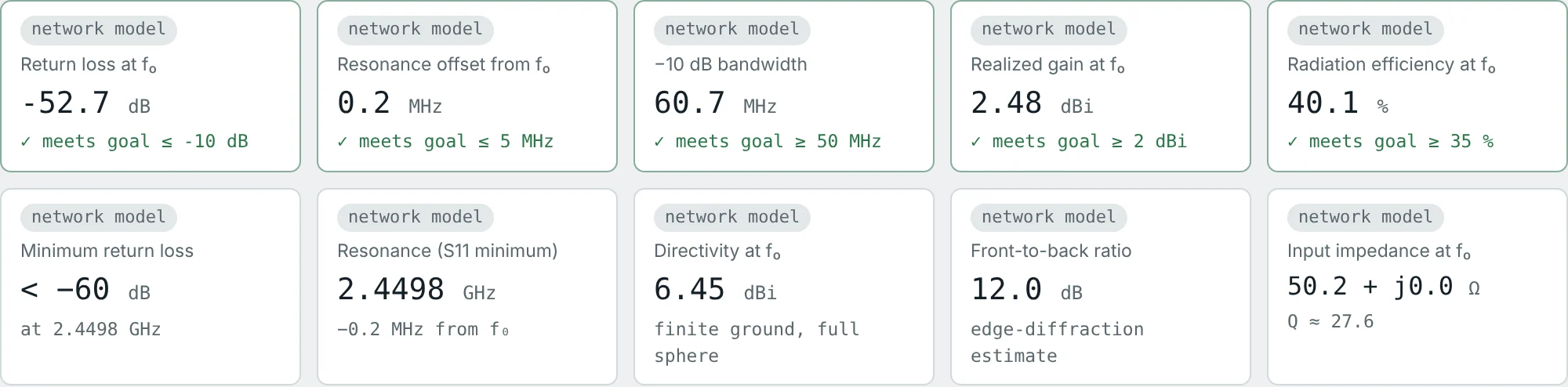
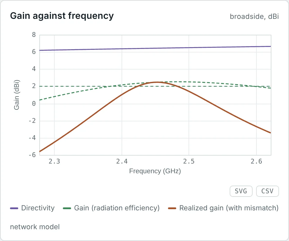
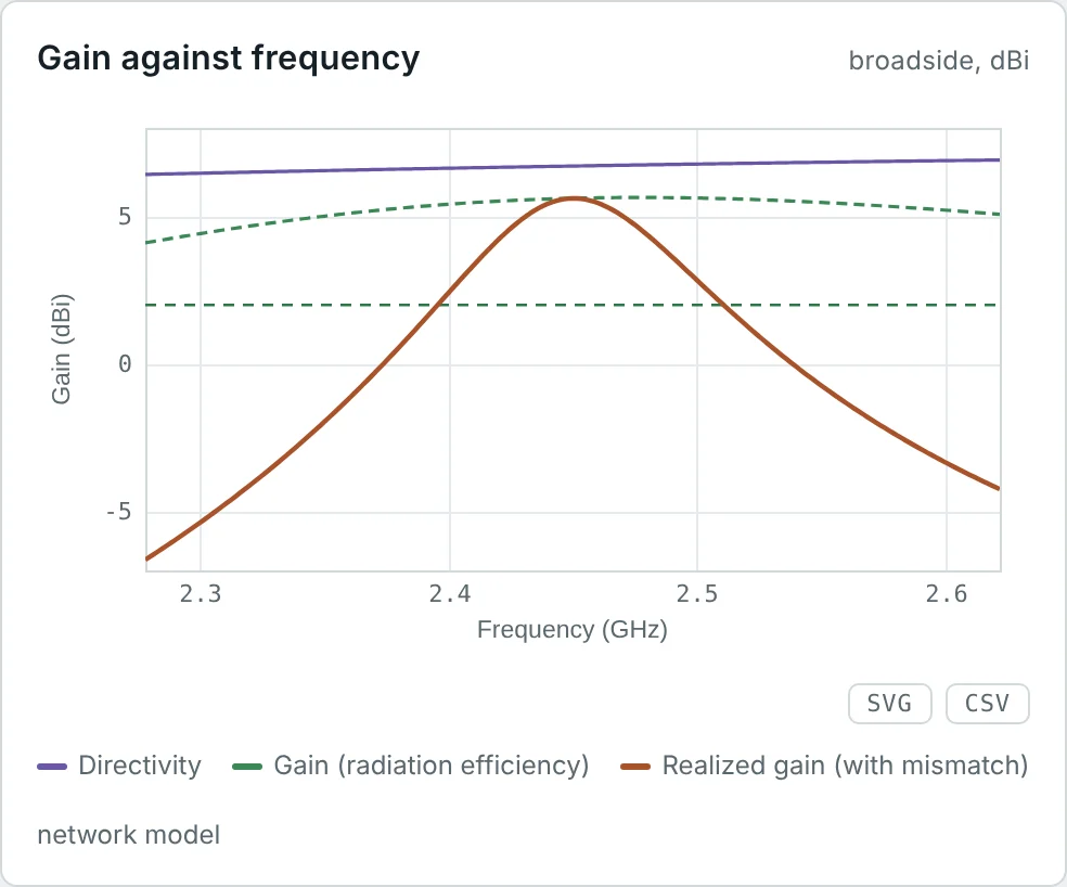
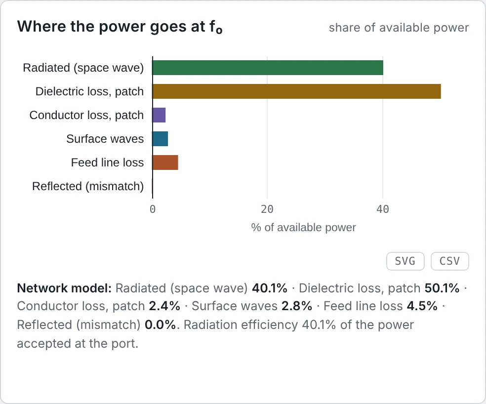
The two patch designs from Part 4 show this clearly. Both are 2.45 GHz inset-fed patches with almost the same pattern — but one is on lossy FR-4 (tan δ = 0.02) and the other on Rogers RO4003C (tan δ = 0.0027):

Gain against frequency for the FR-4 patch: directivity about 6.4 dBi, gain about 2.5 dBi, realized gain peaking at 2.48 dBi at 2.45 GHz — FR-4 patch: the directivity line (purple) sits near 6.4 dBi, but the gain (green, dashed) is only about 2.5 dBi — 4 dB is lost in the substrate. Try it in the Patch Antenna Calculator →

Gain against frequency for the Rogers patch: directivity about 6.7 dBi and gain about 5.6 dBi — Rogers RO4003C patch: directivity 6.72 dBi and gain 5.63 dBi, only about 1.1 dB apart. Try it in the Patch Antenna Calculator →

Power budget of the FR-4 patch: 40.1 percent radiated, 50.1 percent lost in the dielectric, the rest in conductors, surface waves and the feed line — Where the power goes in the FR-4 patch: half of it heats the substrate. That loss — not the pattern — is why its gain is so much lower than its directivity. Try it in the Patch Antenna Calculator →

Gain in dBi and dBd

Gain can be quoted against two references. dBi is relative to an isotropic radiator; dBd is relative to a lossless half-wave dipole, whose gain is 2.15 dBi:

Converting between references

G_{dBi} = G_{dBd} + 2.15

Always check which reference a datasheet uses: the same antenna is "8 dBi" or "5.85 dBd". Link budgets and the Friis equation (Part 13) use dBi.

Realized Gain

Gain is defined with the power the antenna accepts. If the antenna is not perfectly matched to its feed line, part of the available power is reflected before it ever reaches the antenna (Part 8). Realized gain includes this mismatch:

Realized gain

G_{r} = (1 - {| Γ |}^{2}) e_{c d} D_{0} = e_{0} D_{0}

e₀ = (1 − |Γ|²) e_cd is the total efficiency. Realized gain is what the system actually sees and what an over-the-air test measures.

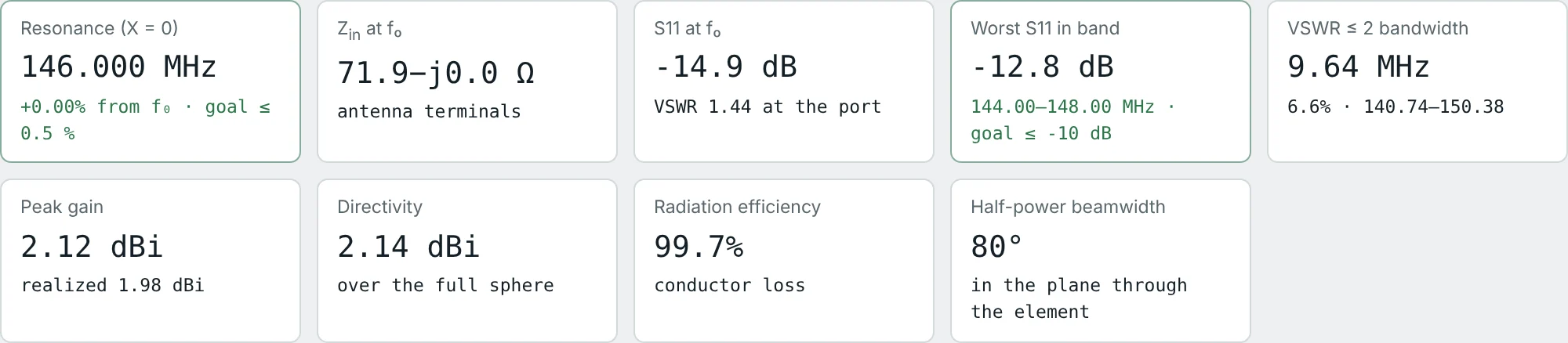
The Method of Moments dipole from Part 4 illustrates all three quantities at once:

Dipole calculator results: peak gain 2.12 dBi, realized 1.98 dBi, directivity 2.14 dBi, radiation efficiency 99.7 percent, S11 minus 14.9 dB — The copper half-wave dipole at 146 MHz: directivity 2.14 dBi, radiation efficiency 99.7% (gain 2.12 dBi), and S11 = −14.9 dB on a 50 Ω port, giving a realized gain of 1.98 dBi. Try it in the Dipole & Monopole Antenna Calculator →

Partial Directivity and Polarization

The far field has two orthogonal components, E_θ and E_φ (Part 4), and the radiation intensity is the sum of their contributions, U = U_θ + U_φ. Directivity splits the same way into partial directivities:

Partial directivities

D_{θ} = \frac{4 π U_{θ}}{P_{rad}} D_{φ} = \frac{4 π U_{φ}}{P_{rad}} D_{0} = D_{θ} + D_{φ}

Note that P_rad in each denominator is the total radiated power. For a linearly polarized antenna the wanted (co-polar) partial directivity is almost the total; the remainder is cross-polarization, which Part 11 treats in detail.

Partial directivity matters whenever only one polarization is received. A receiver with a vertical antenna sees only the partial directivity of the vertical component of the transmitter, not its total directivity — one source of the polarization mismatch loss in link budgets.

How Large Can Directivity Be?

Directivity grows with antenna size in wavelengths, and two results bound it from above. For a planar aperture of physical area A, the highest directivity is obtained with uniform illumination:

Aperture limit

D_{max} = \frac{4 π A}{λ^{2}} D_{0} = ε_{ap} \frac{4 π A}{λ^{2}}

ε_ap is the aperture efficiency, typically 0.5–0.8 for dishes and horns. Tapering the illumination to lower the side lobes (Part 4) reduces ε_ap. Part 12 develops this as the effective aperture A_e = Dλ²/4π.

For an antenna of any shape that fits inside a sphere of radius a, Harrington showed that the "normal" maximum directivity — achievable without impractically large currents and losses — is approximately

Harrington's normal-gain limit

D_{normal} \approx {(k a)}^{2} + 2 k a

A half-wave dipole (a = λ/4, ka = π/2) could in principle reach 5.6 (7.5 dBi), but its simple standing-wave current gives only 1.64. Designs that exceed the normal limit ("superdirective" arrays) need closely spaced elements with large opposing currents, very high Q and very low efficiency — so gain, not directivity, ends up limited.

Antenna Gain Measurement

Gain is measured in an anechoic chamber or on a far-field range. Both standard methods are built on the Friis transmission equation (Part 13), which in decibels for two antennas a distance R apart reads

Friis equation in dB — the basis of every gain measurement

G_{t} + G_{r} = 20 \log_{10} (\frac{4 π R}{λ}) + 10 \log_{10} (\frac{P_{r}}{P_{t}})

Valid in the far field of both antennas, with matched polarization and impedance (or with those losses corrected separately).

Gain-Transfer (Comparison) Method

Measure the received power with a reference antenna of known gain G_ref — usually a calibrated standard-gain horn — then replace it with the antenna under test (AUT) in exactly the same position. Everything else in the Friis equation is unchanged, so it cancels:

Gain-transfer equation

G_{AUT} (dBi) = G_{ref} (dBi) + P_{AUT} (dBm) - P_{ref} (dBm)

Three-Antenna Method

When no calibrated reference exists, measure the transmission between each pair of three antennas A, B and C at a known distance. Each measurement gives one equation in the sum of two gains:

Three equations, three unknowns

G_{A} + G_{B} = S_{A B} G_{A} + G_{C} = S_{A C} G_{B} + G_{C} = S_{B C} G_{A} = \frac{S_{A B} + S_{A C} - S_{B C}}{2}

S_ij is the right-hand side of the Friis equation for that pair. G_B and G_C follow by symmetry. National measurement laboratories use this method to calibrate the standard-gain horns that everyone else uses as references.

Directivity is obtained by integrating a full 3D pattern measurement with the formula for D₀ above; dividing gain by directivity then gives the radiation efficiency. Electrically small antennas are often measured in reverberation chambers or Wheeler caps, which measure efficiency directly (Part 9).

Numerical Examples of Directivity and Gain

Directivity From Radiation Intensity

Problem: An antenna radiates 10 W. Its maximum radiation intensity is 5 W/sr. Find U₀, D₀ (linear and dBi) and the power density at 1 km, isotropic and on the main beam.

U_{0} = \frac{10}{4 π} = 0.796 W/sr D_{0} = \frac{5}{0.796} = 6.28 = 7.98 dBi S_{0} = \frac{10}{4 π {(1000)}^{2}} = 0.796 µW/m²

Answer: U₀ = 0.796 W/sr, D₀ = 6.28 (7.98 dBi)

On the main beam at 1 km the power density is U_max/r² = 5.0 µW/m² — exactly D₀ × S₀. The equivalent beam solid angle is Ω_A = 4π/6.28 = 2.0 sr.

A Short Dipole: Directivity and Radiation Resistance

Problem: A 2 cm element at 300 MHz (L = λ/50) carries 1 A peak. Find its directivity, radiation resistance and radiated power.

D_{0} = 1.5 R_{r} = 80 π^{2} {(\frac{1}{50})}^{2} = 0.316 Ω P_{rad} = \frac{1}{2} I^{2} R_{r} = 0.158 W

Answer: D₀ = 1.5 (1.76 dBi), R_r = 0.32 Ω, P_rad = 0.16 W

The directivity is respectable, but with a radiation resistance of a third of an ohm, even 1 Ω of conductor loss would waste three-quarters of the power. Small antennas are limited by efficiency, not directivity.

Directivity of a Half-Wave Dipole

Problem: Using U_max = ηI₀²/(8π²) and P_rad = ηI₀²Cin(2π)/(8π) with Cin(2π) = 2.4377, find D₀, P_rad for I₀ = 1 A, and R_r.

U_{max} = \frac{120 π}{8 π^{2}} = 4.775 W/sr P_{rad} = 15 \times 2.4377 = 36.57 W D_{0} = \frac{4 π \times 4.775}{36.57} = 1.641

Answer: D₀ = 1.64 = 2.15 dBi, P_rad = 36.6 W, R_r = 2P_rad/I₀² = 73.1 Ω

The calculator's Method of Moments solution for a real 2 mm copper wire gives 2.14 dBi and 72 Ω at resonance — the thin-wire theory and the full solver agree closely. Part 7 explains the small difference in resistance.

Designing a Beam for 10 dBi

Problem: A feed antenna has a cosⁿθ pattern in its forward hemisphere. Which n gives 10 dBi directivity? What is its HPBW, and how well does the Kraus formula predict D₀?

2 (n + 1) = 10 \Rightarrow n = 4 \cos^{4} θ_{h} = 0.5 \Rightarrow θ_{h} = 32.8 °, HPBW = 65.5 ° D_{Kraus} = \frac{41253}{{65.5}^{2}} = 9.61

Answer: n = 4, HPBW = 65.5°, Kraus estimate 9.61 (9.83 dBi) against the exact 10.00 (10 dBi)

A 0.17 dB error is excellent for a two-number estimate. For this broad beam the Tai–Pereira formula gives 8.48 (9.3 dBi) — less accurate here.

Directivity of an Eight-Element Array

Problem: Eight isotropic elements are spaced λ/2 apart in a broadside array. Find D₀ and check it against the long-array formula and the beamwidth from Part 4.

D_{0} = N = 8 = 9.03 dBi \frac{2 N d}{λ} = \frac{2 \times 8 \times 0.5 λ}{λ} = 8

Answer: D₀ = 8 (9.03 dBi)

The beam is a 12.8° fan in the plane of the array but omnidirectional around its axis, so the Kraus formula — which assumes a pencil beam — does not apply. Directivity comes from narrowing in one plane only, which is why it grows only as N, not N².

Directivity of a Horn From Its Beamwidths

Problem: A horn has a 30° half-power beamwidth in both principal planes. Estimate its directivity with both formulas.

D_{Kraus} = \frac{41253}{30 \times 30} = 45.8 = 16.6 dBi D_{TP} = \frac{72815}{900 + 900} = 40.5 = 16.1 dBi

Answer: about 16–16.6 dBi

For narrow beams the two estimates agree within half a decibel; measurement or simulation settles the final figure.

Gain of an FR-4 and a Rogers Patch

Problem: The FR-4 patch has D₀ = 6.45 dBi and e_cd = 40.1%; the Rogers patch has D₀ = 6.72 dBi and e_cd = 77.7%. Find the gain of each.

G_{FR-4} = 6.45 + 10 \log 0.401 = 6.45 - 3.97 = 2.48 dBi G_{Rogers} = 6.72 - 1.10 = 5.62 dBi

Rogers patch calculator results: realized gain 5.63 dBi, radiation efficiency 77.7 percent, directivity 6.72 dBi, bandwidth 33.9 MHz — Rogers RO4003C results from the calculator: 5.63 dBi realized gain from 6.72 dBi directivity at 77.7% efficiency. Note the narrower 33.9 MHz bandwidth — loss broadens bandwidth, a trade-off explored in Part 10. Try it in the Patch Antenna Calculator →

Answer: 2.48 dBi on FR-4, 5.62 dBi on Rogers — 3.1 dB more gain from a better substrate

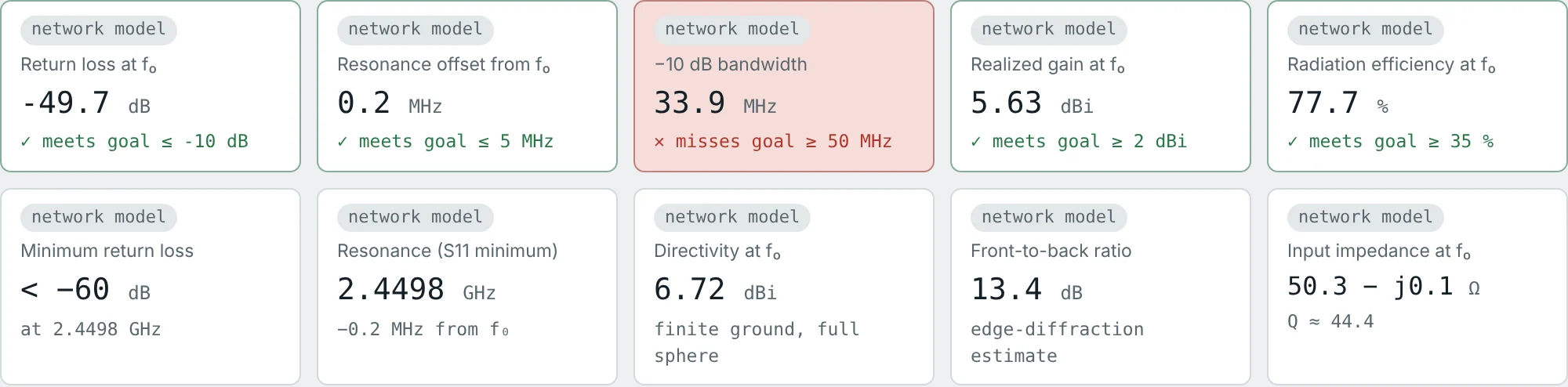
The directivities differ by only 0.27 dB. Almost the entire gain difference is efficiency. Both directivities fit a cosⁿ pattern with n ≈ 1.2–1.4 (D₀ = 2(n + 1) = 4.4–4.7).

Realized Gain and dBd of the Dipole

Problem: The copper dipole has G = 2.12 dBi and S11 = −14.9 dB at its 50 Ω port. Find its realized gain, its gain in dBd, and its total efficiency.

{| Γ |}^{2} = 10^{- 1.49} = 0.032 G_{r} = 2.12 + 10 \log (0.968) = 1.98 dBi G_{dBd} = 2.12 - 2.15 = - 0.03 dBd

Answer: realized gain 1.98 dBi; gain −0.03 dBd; total efficiency e₀ = 0.968 × 0.997 = 96.5%

A real copper dipole is 0.03 dB below the ideal lossless dipole that defines 0 dBd. The 72 Ω dipole on a 50 Ω port loses a further 0.14 dB to mismatch — Part 7 explains where the 72 Ω comes from.

Gain-Transfer Measurement

Problem: In a chamber, a standard-gain horn of 15.0 dBi receives −42.3 dBm. The antenna under test, placed in the same position and aligned for maximum signal, receives −45.1 dBm. Both are matched. Find the AUT gain.

G_{AUT} = 15.0 + (- 45.1) - (- 42.3) = 12.2 dBi

Answer: 12.2 dBi

If the AUT had a VSWR of 2 (|Γ|² = 0.111), the same reading would be its realized gain; its gain would be 12.2 + 0.51 = 12.7 dBi. Always state which one a measurement reports.

Calibrating Three Antennas Without a Reference

Problem: Three horns are measured in pairs at R = 3 m and 10 GHz (λ = 3 cm). The received-to-transmitted power ratios are −41.0 dB (A–B), −38.5 dB (A–C) and −40.1 dB (B–C). Find all three gains.

20 log₁₀(4πR/λ) = 20 log₁₀(1256.6) = 61.98 dB

S_{A B} = 20.98 S_{A C} = 23.48 S_{B C} = 21.88 G_{A} = \frac{20.98 + 23.48 - 21.88}{2} = 11.29 dBi

Answer: G_A = 11.3 dBi, G_B = 9.7 dBi, G_C = 12.2 dBi

Check: G_A + G_B = 20.98 ✓, G_A + G_C = 23.48 ✓, G_B + G_C = 21.88 ✓. At 3 m the far-field condition 2D²/λ ≥ R limits the horn aperture to D ≤ 21 cm.

Summary

Directivity D₀ = 4πU_max/P_rad compares the peak radiation intensity with that of an isotropic source radiating the same power.
It depends only on the pattern shape: 1.5 (1.76 dBi) for a short dipole, 1.64 (2.15 dBi) for a half-wave dipole.
Gain G = e_cd·D₀ includes conductor and dielectric losses; realized gain also includes mismatch: G_r = (1 − |Γ|²)·G.
Directivity splits into partial directivities for the two polarizations, and is bounded by 4πA/λ² for an aperture and by about (ka)² + 2ka for an antenna inside a sphere of radius a.
dBi is relative to isotropic, dBd to a half-wave dipole: dBi = dBd + 2.15.
D₀ = 4π/Ω_A: a short dipole gives 1.5, a half-wave dipole 4/Cin(2π) = 1.64, a cosⁿ pattern 2(n + 1), and a λ/2-spaced array of N elements N.
Directivity can be estimated from beamwidths (≈ 41 253/θ_Eθ_H) and gain is measured by comparison or the three-antenna method.

Gain depends on how much of the input power the antenna accepts, and that depends on its impedance. Part 7: Antenna Input Impedance and Radiation Resistance looks at the antenna from its terminals.

Put It Into Practice

Use the NEXT ANTENNAS calculators to apply the ideas from this article to real antennas.

Wire Antennas Dipole & Monopole Antenna Calculator Method of Moments design of dipoles, inverted-Vs and monopoles: length, impedance, S11, current, gain and 3D patterns. Open calculator → Antenna Design Patch Antenna Calculator Microstrip patch synthesis and simulation: dimensions, feed, S11, gain, efficiency and radiation patterns. Open calculator → Link & Power Link Budget Calculator Transmit power, antenna gains, path loss and margin for a complete wireless link. Open calculator → All Tools All RF Calculators Browse every NEXT ANTENNAS calculator for RF, microwave and antenna design. Open calculator →

Antenna Directivity and Gain