Antenna Near Field and Far Field Explained

Fig 1 — The three field regions of an antenna of largest dimension D. The boundaries are conventions based on how much phase error is acceptable, not sharp physical walls

Introduction to Antenna Field Regions

Part 2 showed that the exact field of a short dipole contains three kinds of terms, falling as 1/r³, 1/r² and 1/r. Close to the antenna, the fast-decaying terms dominate and the field is mostly stored energy; far away, only the 1/r radiation term is left. For an antenna that is large compared with the wavelength — a dish, a horn, an array — there is a second effect: the distances from different parts of the antenna to the observer differ, and those path differences change the way the contributions add.

Both effects are captured by dividing the space around the antenna into three regions, standardized in IEEE 145:

Reactive near fieldImmediately around the antenna, where reactive (stored) energy dominates over radiated energy.

Radiating near fieldRadiation dominates, but the angular distribution still depends on distance. Also called the Fresnel region.

Far fieldThe angular field distribution no longer depends on distance. Also called the Fraunhofer region.

Everything quoted on a datasheet — pattern, beamwidth, gain, polarization — is a far-field quantity. Knowing where the far field starts is therefore essential for measuring antennas, for predicting RF exposure, and for understanding when the Friis equation of Part 13 can be trusted.

Where the Boundaries Come From

Consider an antenna of largest dimension D, with a source point at distance r′ from its centre (r′ ≤ D/2), and an observer at distance r in a direction making an angle ψ with the line to the source point. The exact distance between them is

Distance from a source point to the observer — binomial expansion

R = \sqrt{r^{2} + {r'}^{2} - 2 r r' \cos ψ} = r - r' \cos ψ + \frac{{r'}^{2} \sin^{2} ψ}{2 r} + \frac{{r'}^{3} \cos ψ \sin^{2} ψ}{2 r^{2}} + \dots

In the radiation integral A = (μ/4π)∫J e^(−jkR)/R dV, R in the denominator only affects amplitude and can be replaced by r. R in the exponent sets the phase and must be approximated much more carefully, because an error of λ/2 in R reverses the sign of a contribution.

Fig 2 — Geometry of the far-field approximation: rays from the centre and the edge of an aperture to a distant observer differ in length by r′cos ψ plus a small quadratic term

The far-field (Fraunhofer) distance

The far-field approximation keeps R ≈ r − r′cos ψ in the phase, which treats the rays from all source points as parallel. The first neglected term, r′² sin²ψ/(2r), is largest at ψ = 90° and at the edge of the antenna, r′ = D/2. The accepted criterion, used by IEEE, is that this term may cause a phase error of at most π/8 (22.5°):

Derivation of the Fraunhofer distance

k \frac{{(D / 2)}^{2}}{2 r} = \frac{2 π}{λ} \cdot \frac{D^{2}}{8 r} \leq \frac{π}{8} \Rightarrow R_{2} = \frac{2 D^{2}}{λ}

The Fraunhofer (Rayleigh) distance. At r = 2D²/λ the edge ray is longer than the parallel-ray estimate by D²/8r = λ/16. For a uniformly illuminated aperture this error lowers the measured gain by about 0.1 dB and fills in the first nulls slightly.

Two extra conditions apply. The derivation assumed r ≫ D (so the amplitude 1/R ≈ 1/r) and, implicitly, r ≫ λ (so the reactive 1/r² and 1/r³ terms of Part 2 have died away). For electrically small antennas, where 2D²/λ is smaller than λ, those other conditions set the far-field boundary:

Complete far-field conditions

r > \frac{2 D^{2}}{λ} and r ≫ D and r ≫ λ

"≫" is commonly taken as a factor of 5 to 10. For a half-wave dipole, the last condition (r of several wavelengths) is the one that matters.

The reactive near-field boundary

Inside the Fresnel region the quadratic term is kept, and the approximation fails when the next term, the cubic r′³ cos ψ sin²ψ/(2r²), becomes significant. The function cos ψ sin²ψ is largest at tan ψ = √2 (ψ = 54.7°), where it equals 2/(3√3) = 0.385. Applying the same π/8 criterion at r′ = D/2:

Derivation of the reactive near-field boundary

\frac{2 π}{λ} \cdot \frac{{(D / 2)}^{3} \times 0.385}{2 r^{2}} \leq \frac{π}{8} \Rightarrow r^{2} \geq 0.385 \frac{D^{3}}{λ} \Rightarrow R_{1} = 0.62 \sqrt{\frac{D^{3}}{λ}}

This is the outer boundary of the reactive near field for an antenna large compared with λ. For electrically small antennas (D ≪ λ) the reactive region instead extends to about λ/2π, where the reactive and radiating terms of Part 2 are equal.

Region	Inner boundary	Outer boundary	Applies to
Reactive near field	Antenna surface	0.62 √(D³/λ) — or λ/2π if D ≪ λ	All antennas
Radiating near field (Fresnel)	0.62 √(D³/λ)	2D²/λ	Antennas with D ≳ λ; may not exist for very small antennas
Far field (Fraunhofer)	2D²/λ (and r ≫ D, r ≫ λ)	Infinity	All antennas

The Reactive Near-Field Region

Close to the antenna the fields are dominated by stored energy, which flows out and back each cycle like the energy in a capacitor or inductor. Its characteristics:

E and H are roughly 90° out of phase, so the time-average Poynting vector carried by these terms is zero. The complex Poynting vector is mostly imaginary (reactive power).
Fields have radial components. For a short dipole E_r is comparable with or larger than E_θ (Example 7); the field is not a transverse wave.
The wave impedance is not 377 Ω. It is high and capacitive near electric sources (dipoles, monopoles) and low and inductive near magnetic sources (loops, slots fed as loops) — Fig 2 of Part 2.
Fields fall off fast, as 1/r² to 1/r³, so they are strong close to the antenna and negligible a short distance away.
Nearby objects interact strongly. A hand, a metal case or a tissue layer in this region couples to the stored energy and changes the input impedance and resonant frequency. This is why a phone antenna detunes when held, and why the reactive near field is part of the antenna's "keep-out" volume in product design.

How much energy is stored? The complex power of a dipole

The exact fields of the Hertzian dipole (Part 2) let us compute the complex power flowing through a sphere of radius r. Integrating the complex Poynting vector ½E × H* over the sphere, only E_θH_φ* contributes to the radial flow:

Complex power through a sphere around a short dipole — derivation

P = \frac{1}{2} \int_{0}^{2 π} \int_{0}^{π} E_{θ} H_{φ}^{*} r^{2} \sin θ d θ d φ = \frac{η π}{3} {| \frac{I L}{λ} |}^{2} [1 - j \frac{1}{{(k r)}^{3}}]

Multiplying the bracket of E_θ, [1 + 1/(jkr) − 1/(kr)²], by the conjugate of the bracket of H_φ, [1 − 1/(jkr)], the cross terms cancel and leave 1 − j/(kr)³. The real part, the radiated power, is the same through every sphere. The imaginary (capacitive) part is the reactive power stored outside radius r; it grows as 1/(kr)³ as the sphere shrinks towards the antenna.

The ratio of reactive to radiated power through a sphere of radius a is 1/(ka)³. If the antenna fits inside that sphere, this ratio is a lower bound on its quality factor Q, and therefore an upper bound on its bandwidth. This is the physical origin of the Chu limit that restricts small antennas, developed in Part 10: the reactive near field is not a nuisance to be designed away, it is unavoidable stored energy.

Fig 3 — Magnitudes of the three terms in E_θ of a short dipole (common factor ηkIL sin θ/4π removed, multiplied by 1/r): the quasi-static term dominates below kr = 1, the radiation term above

quasi-static 1/(kr)³induction 1/(kr)²radiation 1/(kr)

The Radiating Near-Field (Fresnel) Region

Between R₁ and R₂ the radiation terms dominate, so power flows outward, but the quadratic phase term r′² sin²ψ/2r is still significant. Contributions from different parts of the antenna arrive with phase differences that depend on r, so the shape of the pattern changes with distance:

Measured main beams are broader and nulls are filled in compared with the far field.
Close to a large aperture, the power flows in a roughly collimated beam about as wide as the aperture itself — the field has not yet "spread" (Example 9).
The measured on-axis gain is lower than the far-field gain and oscillates with distance for uniform apertures.
The field is predominantly transverse, and |E|/|H| is close to 377 Ω.

For a small antenna such as a half-wave dipole, R₁ and R₂ are both comparable with λ, and the radiating near field is a thin shell or does not exist at all; the field goes straight from reactive to far-field behaviour around r ≈ λ/2π to a few λ.

The Far-Field (Fraunhofer) Region

Beyond R₂ (and many D and λ away) the field from any antenna takes the universal form derived in Part 2:

Far-field properties

E = \frac{e^{- j k r}}{r} F (θ, φ) E_{r} \approx 0 H = \frac{\hat{r} \times E}{η} S_{av} = \frac{{| E |}^{2}}{2 η} \hat{r}

The angular dependence F(θ, φ) is independent of r: this is the definition of the far field. Radiation patterns, directivity, gain and polarization are all defined from F.

The wave is locally plane: E, H and the direction of travel are mutually perpendicular, in phase, with |E|/|H| = η = 377 Ω.
Field strength falls as 1/r and power density as 1/r² — the inverse-square law.
Measurements of E alone are enough to know H and the power density, which simplifies RF surveys.
The Friis transmission equation (Part 13) and the gain of Part 6 are valid only here.

Electric and Magnetic Field Relationships in Each Region

Property	Reactive near field	Radiating near field	Far field
Dominant energy	Stored (reactive)	Radiated	Radiated
Phase between E and H	≈ 90°	Nearly in phase	In phase
Radial components	Significant	Small	Negligible
Wave impedance \|E\|/\|H\|	≫ 377 Ω (electric source) or ≪ 377 Ω (magnetic source)	≈ 377 Ω	377 Ω
Distance dependence	1/r² – 1/r³	Roughly 1/r, with oscillations	Exactly 1/r
Pattern shape	Not defined	Changes with r	Independent of r
What to measure for exposure	E and H separately	E or H, with care	E (H and S follow)

Wavelength and Antenna Dimensions

Because R₂ grows as D²/λ, the far-field distance of electrically large antennas becomes enormous at high frequency. The table shows how strongly the regions depend on size in wavelengths:

Antenna	D	f	λ	R₁ = 0.62√(D³/λ)	R₂ = 2D²/λ
Half-wave dipole	0.98 m	146 MHz	2.05 m	(use λ/2π = 0.33 m)	0.94 m (use several λ instead)
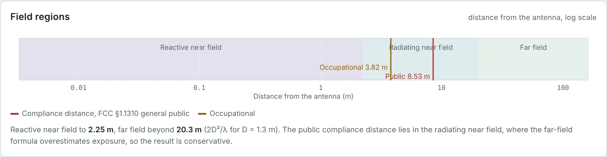
Cellular panel	1.3 m	1.8 GHz	16.7 cm	2.25 m	20.3 m
Satellite TV dish	1.2 m	12 GHz	2.5 cm	5.16 m	115 m
28 GHz 5G array	10 cm	28 GHz	10.7 mm	0.19 m	1.87 m
Radio telescope dish	25 m	1.42 GHz	21.1 cm	169 m	5.9 km

Field regions bar from the RF exposure calculator: reactive near field to 2.25 metres, radiating near field to 20.3 metres, far field beyond, with the public and occupational compliance distances marked — Field regions of a 1.3 m, 1800 MHz cellular panel in the RF Exposure Calculator: reactive near field to 2.25 m, far field beyond 20.3 m. The public compliance distance (8.5 m) falls in the radiating near field. Try it in the RF Exposure Calculator →

Near-Field vs. Far-Field Measurements

Antenna patterns and gain are far-field quantities, but measuring at 2D²/λ is impractical for large or high-frequency antennas. Three families of test range exist:

Method	Principle	Strengths	Limitations
Far-field range (outdoor, anechoic chamber)	Source at r ≥ 2D²/λ illuminates the antenna under test with a near-plane wave	Direct, simple processing	Long distance for large D; ground reflections; weather
Compact antenna test range (CATR)	A large reflector turns a spherical wave into a plane wave over a "quiet zone"	Far-field conditions in a few metres; real-time pattern cuts	Expensive reflector; quiet-zone size limits the antenna size
Near-field scanning (planar, cylindrical, spherical)	A probe samples amplitude and phase on a surface 3–5 λ from the antenna; the far field is computed by a modal (Fourier) transform	Small chamber, full 3D information, diagnostics of aperture fields	Requires phase-stable measurement and λ/2 sampling; probe correction

Near-field scanners work because the radiating near field contains the complete information about the far field: the transform is just the exact version of the "add up all the contributions" integral, without the parallel-ray approximation. The sampling theorem requires a grid spacing of at most λ/2 (Example 6).

Practical Applications of Different Field Regions

Field region	Application	Why that region
Reactive near field	NFC, HF RFID, Qi wireless charging, inductive hearing loops	Strong coupling at short range; the field dies off quickly so there is little interference or eavesdropping
Reactive near field	Antenna detuning, SAR in phones, EMC near-field probes	Objects in the stored-energy region change impedance or absorb power
Radiating near field	Near-field antenna measurement, microwave imaging, some UHF RFID portals	Complete field information in a small volume
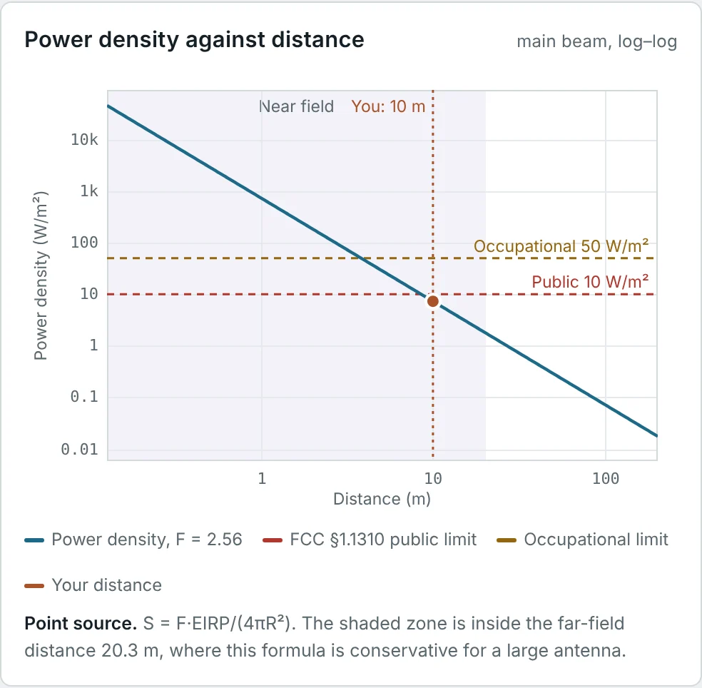
Radiating near field	RF exposure around base stations and broadcast towers	Public areas are often within 2D²/λ of large panels; far-field formulas over-estimate exposure here, so they are conservative
Far field	All communication links, radar, broadcasting	Gain and pattern are stable; Friis and radar equations apply

RF-exposure standards (FCC OET-65, ICNIRP) recognize the regions explicitly: a simple far-field estimate S = EIRP/(4πr²) is allowed everywhere because it over-predicts the power density in the near field of an aperture, while specialist cylindrical-wave models are used close to large panels. The RF Exposure Calculator marks the regions on every result.

Power density against distance for the cellular panel, a straight line on log-log axes with the public and occupational limits and the shaded near-field zone — Power density against distance for the same panel. The straight line is the far-field formula S = F·EIRP/(4πr²); inside the shaded near-field zone (up to 20.3 m) it is an upper bound on the true power density. Try it in the RF Exposure Calculator →

Worked Examples

Field Regions of a Satellite Dish

Problem: A 1.2 m dish operates at 12 GHz. Find R₁ and R₂.

λ = 0.025 m R_{1} = 0.62 \sqrt{\frac{{1.2}^{3}}{0.025}} = 0.62 \times 8.31 = 5.16 m R_{2} = \frac{2 \times {1.2}^{2}}{0.025} = 115 m

Answer: reactive near field to 5.2 m, far field beyond 115 m

A pattern measured 30 m away would be in the radiating near field and would show a broadened beam and filled nulls. Dishes of this size are measured on compact ranges or near-field scanners.

Far-Field Distance of a Half-Wave Dipole

Problem: For a 146 MHz half-wave dipole (D = 0.98 m, λ = 2.05 m), evaluate the three far-field conditions and decide a sensible minimum measurement distance.

\frac{2 D^{2}}{λ} = \frac{2 \times {0.98}^{2}}{2.05} = 0.94 m r ≫ D : r ≳ 5 m r ≫ λ : r ≳ 10 m

Answer: 2D²/λ is only 0.94 m, but r ≫ λ requires about 10 m

For antennas comparable with or smaller than λ, 2D²/λ is not the binding condition. A good rule for small antennas is r ≥ 3λ–10λ, depending on the accuracy needed.

Base-Station Panel and RF Exposure

Problem: A 1.3 m cellular panel at 1800 MHz has a public compliance distance of 8.53 m (calculator result, FCC limit). In which region is that distance, and is the far-field formula optimistic or conservative there?

R_{1} = 0.62 \sqrt{\frac{{1.3}^{3}}{0.1666}} = 2.25 m R_{2} = \frac{2 \times {1.3}^{2}}{0.1666} = 20.3 m

Answer: 2.25 m < 8.53 m < 20.3 m — the radiating near field; the far-field formula is conservative

In the Fresnel region the power is spread over roughly the panel's own vertical extent rather than concentrated by its full far-field gain, so the true on-axis power density is lower than EIRP/(4πr²).

Phase Error at Shorter Distances

Problem: Find the maximum quadratic phase error across an aperture at r = 2D²/λ, D²/λ and D²/(2λ).

Δ φ = \frac{2 π}{λ} \frac{D^{2}}{8 r} = \frac{π}{4} \cdot \frac{D^{2} / λ}{r} Δ φ = 22.5 °, 45 °, 90 °

Answer: 22.5°, 45° and 90°

At 90° the edge contributions are in quadrature with the centre: the main beam broadens markedly and nulls disappear. Very high-gain or very low-side-lobe antennas are measured at 4D²/λ or more, or with near-field techniques.

A 28 GHz Phased Array

Problem: A 28 GHz array is 10 cm across. Can its far-field pattern be measured in a 3 m anechoic chamber?

λ = 10.7 mm R_{2} = \frac{2 \times {0.1}^{2}}{0.0107} = 1.87 m R_{1} = 0.19 m

Answer: yes — 1.87 m fits in a 3 m chamber

A full base-station array (say 0.5 m at 28 GHz) would need 47 m, which is why 3GPP over-the-air testing of mm-wave equipment uses compact ranges.

Planning a Planar Near-Field Scan

Problem: A 1 m × 1 m scan plane is used to measure an antenna at 10 GHz with λ/2 sampling. How many sample points are needed, and how far from the antenna should the scan plane be?

λ = 3 cm, Δ = \frac{λ}{2} = 1.5 cm N \approx {(\frac{100}{1.5} + 1)}^{2} \approx 68^{2} \approx 4600 d \approx 3 λ - 5 λ = 9 - 15 cm

Answer: about 4 600 points, with the probe 9–15 cm from the antenna

The scan distance keeps the probe out of the reactive near field (so it does not load the antenna) while staying close enough that the scan plane captures nearly all the radiated power.

Radial Field Near a Short Dipole

Problem: Using the exact Hertzian-dipole fields of Part 2, find |E_r|/|E_θ| at kr = 2 and θ = 45°.

\frac{E_{r}}{E_{θ}} = \frac{2 \cos θ}{j k r \sin θ} \frac{1 + \frac{1}{j k r}}{1 + \frac{1}{j k r} - \frac{1}{{(k r)}^{2}}} = \frac{2}{j 2} \cdot \frac{1 - j 0.5}{0.75 - j 0.5} | \dots | = 1 \times \frac{1.118}{0.901} = 1.24

Answer: |E_r| = 1.24 |E_θ| — the radial field is larger than the transverse field at r ≈ 0.32 λ

A field probe oriented only transverse to the line of sight would under-read badly here. Near-field exposure surveys use isotropic (three-axis) probes for this reason.

Wave Impedance 1 m from an NFC Loop

Problem: Predict |E|/|H| at 1 m from a small 13.56 MHz loop in its plane, using Z_w(loop) = η²/Z_w(dipole) from Part 2.

λ = 22.1 m, k r = 0.284 \frac{| Z_{w} |}{η} = 0.307 | Z_{w} | = 116 Ω ∠ 88.7 °

Answer: about 116 Ω, almost purely inductive

A measured E/H ratio far from 377 Ω is the experimental signature of the reactive near field. Using an E-field meter alone and assuming 377 Ω would under-estimate the magnetic exposure here by a factor of 3.3.

The Collimated Beam in Front of a Dish

Problem: A 3 m dish at 10 GHz has a far-field gain of about 48 dBi and radiates 100 W. Compare the far-field formula for the on-axis power density at 50 m with the "collimated beam" estimate S ≈ 4P/(πD²) used by OET-65 for the near field.

R_{2} = \frac{2 \times 9}{0.03} = 600 m S_{FF} = \frac{100 \times 10^{4.8}}{4 π 50^{2}} = 200 W/m² S_{NF} \approx \frac{4 \times 100}{π \times 9} = 14 W/m²

Answer: far-field formula 200 W/m², near-field estimate about 14 W/m²

At 50 m (one twelfth of R₂) the beam is still about as wide as the dish, so the power density cannot exceed roughly P/(aperture area). The far-field formula over-estimates by 14 times, which is safe but very pessimistic.

Compliance Distance of a VHF Station

Problem: A 146 MHz station has a time-averaged EIRP of 79.1 W. Using the FCC ground-reflection factor F = 2.56 and the general-public limit of 2 W/m², find the compliance distance. The antenna is 2.5 m long. In which region is the answer?

r = \sqrt{\frac{F \cdot EIRP}{4 π S_{lim}}} = \sqrt{\frac{2.56 \times 79.1}{4 π \times 2}} = 2.84 m R_{2} = \frac{2 \times {2.5}^{2}}{2.05} = 6.09 m

Answer: 2.84 m, inside the radiating near field (far field beyond 6.1 m) — a conservative result

The RF Exposure Calculator gives the same numbers for its "Amateur VHF base" example. Part 5 derives the power-density formula used here.

Summary

The space around an antenna divides into the reactive near field, the radiating near field (Fresnel) and the far field (Fraunhofer).
The boundaries follow from expanding the path length R in the radiation integral: a π/8 phase criterion on the quadratic term gives 2D²/λ, and on the cubic term gives 0.62√(D³/λ).
For small antennas the boundaries are set instead by λ/2π (reactive) and r ≫ λ, r ≫ D (far field).
In the reactive near field E and H are out of phase, have radial parts and a wave impedance far from 377 Ω; objects there detune the antenna.
In the radiating near field power flows outward but the pattern still changes with distance; near large apertures the beam is collimated.
In the far field the wave is locally plane, |E|/|H| = 377 Ω, and pattern, gain and polarization are defined.
Far-field ranges, compact ranges and near-field scanners all aim to obtain the far field; RF-exposure rules use far-field formulas as conservative bounds in the near field.

With the field regions defined, we can describe how the far field is distributed in direction. Part 4: Antenna Radiation Patterns introduces radiation patterns, lobes and beamwidths.

Put It Into Practice

Use the NEXT ANTENNAS calculators to apply the ideas from this article to real antennas.

Link & Power RF Exposure & MPE Calculator Power density, field strength, near- and far-field regions and safe distances against FCC and ICNIRP limits. Open calculator → Wire Antennas Dipole & Monopole Antenna Calculator Method of Moments design of dipoles, inverted-Vs and monopoles: length, impedance, S11, current, gain and 3D patterns. Open calculator → Antenna & Signal Wavelength / Frequency Calculator Convert between frequency and wavelength in free space and in dielectrics. Open calculator → All Tools All RF Calculators Browse every NEXT ANTENNAS calculator for RF, microwave and antenna design. Open calculator →

Antenna Near Field and Far Field