What Is a Smith Chart?
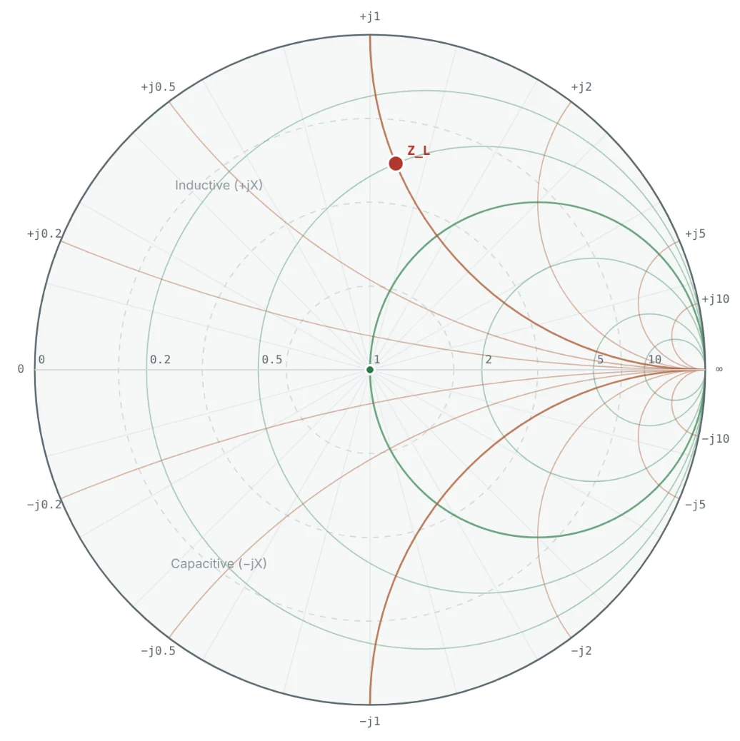
The Smith chart is a graphical calculator for impedance. It is a plot of the complex reflection coefficient Γ (gamma) inside a circle of radius one, overlaid with a grid of circles and arcs that let you read the corresponding impedance directly. Every passive impedance — any combination of resistance, inductance and capacitance — lands on exactly one point inside that circle.
In Part 3 we defined the reflection coefficient as the ratio of the reflected to the incident voltage wave at a load. In Part 5 we saw that moving along a transmission line changes the impedance in a complicated way, but changes Γ in a very simple way: its magnitude stays the same and only its angle rotates. The Smith chart exploits exactly this. By drawing impedance on the Γ plane, line-length problems become rotations, matching problems become moves along circles, and VSWR becomes a radius you can see.
A Smith chart is a polar plot of Γ with the impedance grid z = (1 + Γ)/(1 − Γ) drawn on top, so you can switch between reflection coefficient and impedance just by looking.
History and Development of the Smith Chart
The chart is named after Phillip H. Smith (1905–1987), an engineer at Bell Telephone Laboratories. In the early 1930s Smith was designing antenna feeds and transmission-line matching for radio transmitters, and every calculation of impedance along a line meant laborious work with hyperbolic functions, slide rules and tables. He first drew rectangular charts that plotted impedance against line position; they worked but needed huge sheets, because impedance runs from zero to infinity.
His key insight was to plot the reflection coefficient instead. Because |Γ| ≤ 1 for every passive load, the entire range of impedances fits inside a single circle, and moving along a lossless line is simply a rotation. He published the chart as a "Transmission Line Calculator" in Electronics magazine in January 1939, followed by an improved version in 1944 that added the scales still printed on paper charts today. A very similar chart was published independently in Japan by Tosaku Mizuhashi in 1937, and in Japan it is sometimes called the Mizuhashi–Smith chart.
| Year | Milestone |
|---|---|
| Early 1930s | Smith, at Bell Labs, uses rectangular impedance charts for antenna-feed design |
| 1937 | Tosaku Mizuhashi publishes a circular impedance chart in Japan |
| 1939 | "Transmission Line Calculator" published in Electronics (January) |
| 1944 | "An Improved Transmission Line Calculator" adds the outer wavelength and angle scales |
| 1969 | Smith's book Electronic Applications of the Smith Chart |
| 1970s – today | The chart becomes the standard display of vector network analyzers and RF CAD tools |
Nearly ninety years later, the computer has replaced the paper chart as a calculator, but not as a way of thinking. Every vector network analyzer (VNA) and every RF simulator still displays impedance on a Smith chart, because no other picture shows so much about a match at a glance.
Why Is the Smith Chart Used?
- It fits every impedance on one page. Impedances from 0 to ∞ ohms, inductive or capacitive, all lie inside the unit circle.
- Transmission lines become rotations. Moving a distance d along a lossless line rotates the point by an angle 2βd around the centre. A half wavelength is one full turn.
- Matching becomes geometry. Adding a series reactance moves the point along a circle of constant resistance; adding a shunt reactance moves it along a circle of constant conductance. A matching network is a path from the load to the centre.
- Mismatch is visible. Distance from the centre is |Γ|. Circles around the centre are circles of constant VSWR and return loss.
- Impedance and admittance live on one chart. Rotating a point by 180° converts impedance into admittance, which is what you need for shunt components.
- Frequency behaviour is a curve. A swept measurement traces a curve across the chart, showing at once where a device is matched, how fast it drifts and whether it resonates.
Relationship Between Impedance and Reflection Coefficient
For a load Z_L on a line of characteristic impedance Z₀, the reflection coefficient is fixed by the mismatch between the two. Dividing by Z₀ gives the normalised impedance z = Z_L/Z₀ (the subject of Part 7), and the relationship becomes independent of the system impedance:
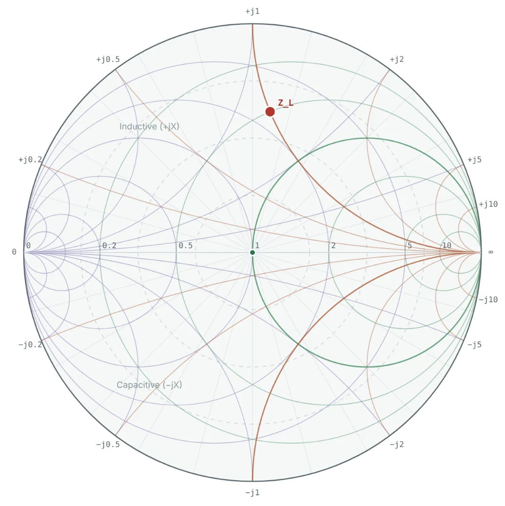
This is a bilinear (Möbius) transformation. It has a remarkable property: it maps circles and straight lines into circles. The whole right half of the impedance plane (all r ≥ 0) maps into the unit disk, every vertical line of constant resistance becomes a circle, and every horizontal line of constant reactance becomes an arc of a circle. That is why the Smith chart is made entirely of circles.
The reflection coefficient, incident and reflected waves and how Γ varies along a line are covered in detail in the transmission line series. Open the Transmission Line Theory series →
Understanding the Smith Chart Geometry
Substituting Γ = u + jv into z = (1 + Γ)/(1 − Γ) and separating real and imaginary parts gives the normalised resistance and reactance at any point on the chart:
The chart is therefore three things laid on top of each other: a polar plot of Γ (magnitude = distance from the centre, angle = direction from the positive u axis), a family of constant-resistance circles, and a family of constant-reactance arcs. Paper charts add outer scales for wavelengths and reflection angle, covered in Part 8.
Resistance and Reactance Circles
Constant-resistance circles
Constant-reactance arcs
A point on the chart is the intersection of one r circle and one x arc. To read an impedance you find which resistance circle and which reactance arc pass through it; to plot an impedance you find the intersection of the circle and arc you want. Part 9 turns this into a step-by-step procedure.
Center Point and Outer Boundary
| Location | Γ | z | Meaning |
|---|---|---|---|
| Centre | 0 | 1 + j0 | Perfect match: Z_L = Z₀, no reflection, VSWR = 1 |
| Left end of the axis | −1 (1∠180°) | 0 | Short circuit |
| Right end of the axis | +1 (1∠0°) | ∞ | Open circuit |
| Horizontal axis | real | r + j0 | Pure resistance: left of centre r < 1, right of centre r > 1 |
| Outer rim | |Γ| = 1 | 0 + jx | Pure reactance (lossless L or C): all power reflected |
| Upper half | v > 0 | x > 0 | Inductive impedance |
| Lower half | v < 0 | x < 0 | Capacitive impedance |
| Outside the rim | |Γ| > 1 | r < 0 | Negative resistance (oscillators, unstable amplifiers) |
The distance from the centre is the magnitude of the mismatch. Points close to the centre are well matched; points near the rim reflect almost all the incident power. Any circle centred on the chart is a circle of constant |Γ| — and therefore of constant VSWR and return loss — which is why the centre is the target of every matching problem.
Applications in RF Engineering
Worked Examples
All examples use a 50 Ω reference impedance. Each one can be reproduced by entering the load in the Smith Chart Calculator.
Plotting a 100 Ω Resistive Load
Problem: Where does a 100 Ω resistor terminating a 50 Ω line appear on the Smith chart? Find Γ and the VSWR.
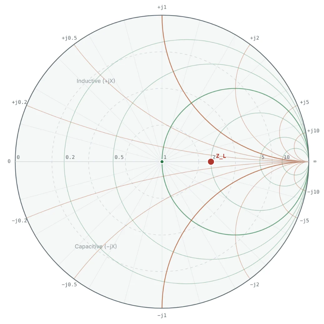
Any pure resistance lies on the horizontal axis. For R > Z₀ the point is right of centre and the VSWR equals r itself (here 2); for R < Z₀ it is left of centre and VSWR = 1/r.
Locating 25 + j50 Ω
Problem: Find Γ for Z_L = 25 + j50 Ω on a 50 Ω line, and show that the point lies on both the r = 0.5 circle and the x = +1 arc.
The point is in the upper half (inductive) and 62% of the way to the rim, so the load is badly mismatched: VSWR = 4.27 and 38% of the incident power is reflected.
From Γ Back to Impedance
Problem: A network analyzer shows Γ = 0.5 ∠ −90° at the end of a 50 Ω cable. What is the load impedance?
An angle of −90° points straight down, into the capacitive lower half — consistent with the negative reactance. At 1 GHz, −j40 Ω corresponds to a series capacitance of 1/(2π × 10⁹ × 40) ≈ 4.0 pF.
Short, Open, Matched and Pure Reactance
Problem: Find Γ for a short circuit, an open circuit, a 50 Ω load, +j50 Ω and −j50 Ω on a 50 Ω line, and locate each on the chart.
| Load | z | Γ | Position (see Fig 4) |
|---|---|---|---|
| Short, 0 Ω | 0 | −1 = 1∠180° | Left end of the axis |
| Open, ∞ | ∞ | +1 = 1∠0° | Right end of the axis |
| 50 Ω | 1 | 0 | Centre |
| +j50 Ω | +j1 | (j − 1)/(j + 1) = +j = 1∠90° | Top of the rim |
| −j50 Ω | −j1 | −j = 1∠−90° | Bottom of the rim |
Lossless reactances reflect all the incident power — they only shift its phase — so they sit on the rim. This is why an ideal inductor or capacitor alone can never be a matched load, but can be used to move a lossy load toward the centre.
Reading r and x From a Point
Problem: A point on the chart has Γ = 0.2 + j0.4. Use the geometry formulas to find r and x, then the impedance in a 50 Ω system.
The point lies on the r = 1 circle — the circle through the centre. That makes it special: adding a series −j50 Ω (a capacitor) would move it along that circle straight to the centre, a one-component match. Points on the r = 1 or g = 1 circles are the stepping stones of every matching design in Parts 10 and 11.
Summary
| Concept | Expression / location | Key point |
|---|---|---|
| Chart coordinates | Γ = u + jv, |Γ| ≤ 1 | Polar plot of the reflection coefficient |
| Impedance ↔ Γ | Γ = (z − 1)/(z + 1), z = (1 + Γ)/(1 − Γ) | Bilinear map: lines become circles |
| Resistance circle | centre (r/(1+r), 0), radius 1/(1+r) | All touch the open-circuit point |
| Reactance arc | centre (1, 1/x), radius 1/|x| | Upper half inductive, lower half capacitive |
| Centre | Γ = 0, z = 1 | Perfect match |
| Rim | |Γ| = 1 | Pure reactance; total reflection |
| Circles about the centre | |Γ| = constant | Constant VSWR and return loss |
- The Smith chart plots the reflection coefficient and overlays the impedance grid, so every passive impedance fits inside one circle.
- It was published by Phillip Smith of Bell Labs in 1939 and remains the standard display of network analyzers and RF CAD tools.
- Constant-resistance lines become circles touching the right edge; constant-reactance lines become arcs.
- The centre is a perfect match, the rim is pure reactance, the upper half is inductive and the lower half capacitive.
The chart is drawn in normalised units. In Part 7: Understanding Normalized Impedance on the Smith Chart we look at why, and how to convert between the chart and real ohms in 50 Ω and 75 Ω systems.
Put It Into Practice
Use the NEXT ANTENNAS calculators to apply the ideas from this article to real designs.