From Theory to the Bench
Over the previous eleven parts we built up impedance, characteristic impedance, Γ, VSWR, line transformation, the chart itself, and matching with lumped elements and stubs. In practice these ideas meet in a few recurring tasks:
- Antenna matching — measure the antenna, then design a network that brings its band into the −10 dB circle.
- Measurement — read a VNA's Smith chart display, recognise resonances, and remove cables and fixtures from the result.
- Amplifier design — choose source and load impedances for gain, noise or stability, using circles drawn on the chart.
- Filters, couplers and passive networks — check input and output match over the band and spot parasitic resonances.
All the examples below use the Smith Chart Calculator with its built-in sample antenna file, so you can reproduce every step.
Matching a Measured Antenna
A VNA saves its measurement as a Touchstone file: an .s1p file for a one-port device such as an antenna, listing frequency and S11 (as magnitude/angle, dB/angle or real/imaginary) at every point. Loading the file into the calculator plots the antenna's impedance at the chosen design frequency and lets the matching solver work on the measured data rather than on a single assumed impedance.
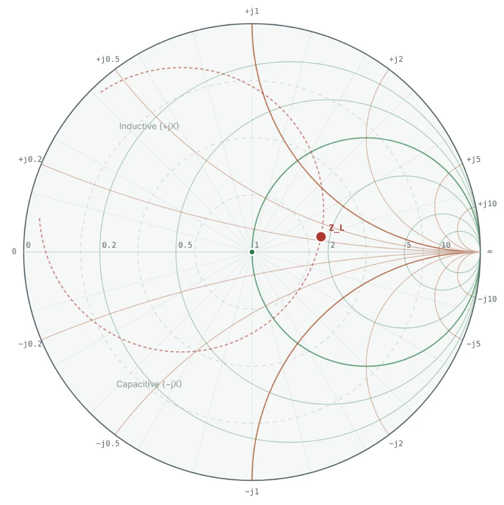
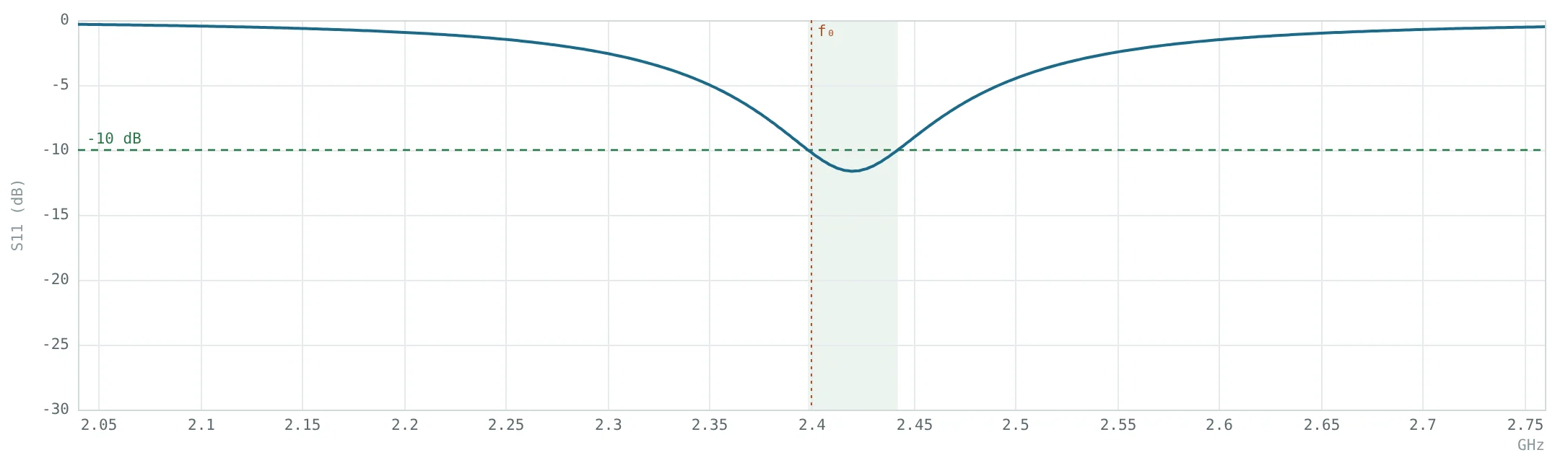

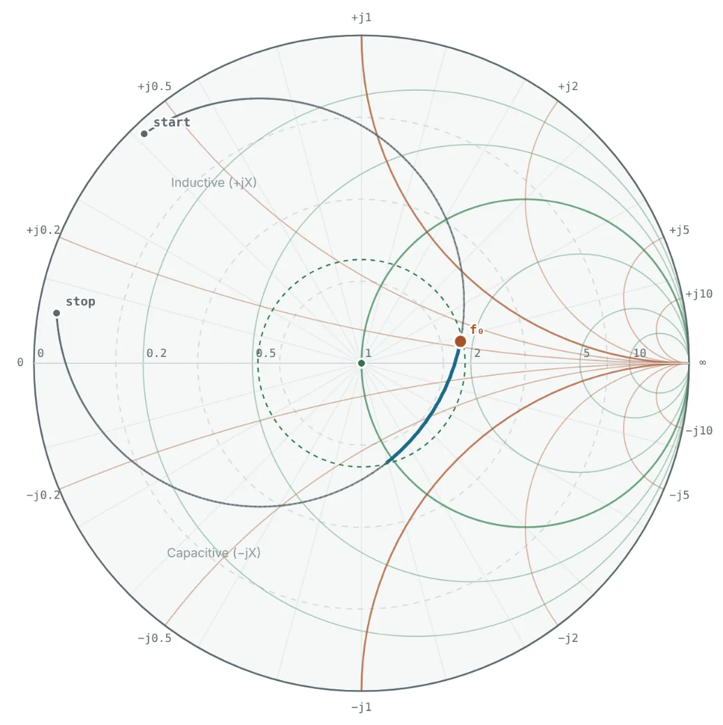
The diagnosis from the chart is immediate: the resonance loop crosses the real axis well to the right of the centre, near z ≈ 1.8 (about 90 Ω), so the antenna's resistance at resonance is too high; and the feed inductance pushes the best match up to 2.42 GHz. Two kinds of fix are possible:
- Change the antenna — move the feed point toward the patch centre to lower the resistance, or lengthen the patch slightly to lower the resonance. On the chart, the loop shrinks toward the centre and rotates so 2.4 GHz lands in the middle of the highlighted section.
- Add a matching network — keep the antenna and transform 92 + j13.6 Ω to 50 Ω at 2.4 GHz. The matching solver finds the options:
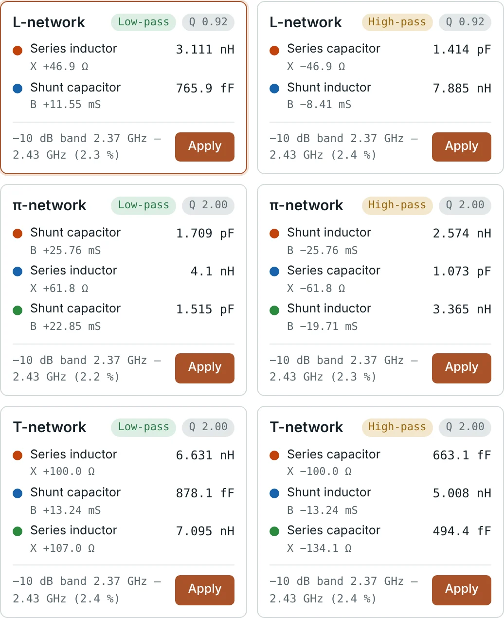
In Part 10 the load was held constant and an L-network achieved up to 105% bandwidth. With a real antenna whose impedance changes rapidly with frequency, every network gives roughly the same 60 MHz band. Matching can centre the band and deepen the null, but it cannot make a high-Q antenna broadband — that requires changing the antenna itself (thicker substrate, different geometry).
Reading Frequency Sweeps on the Chart
On a VNA, S11 is displayed as a trace rather than a point. A few patterns recur:
| Trace shape | Meaning |
|---|---|
| Clockwise motion with increasing frequency | Normal for any passive device (Foster's reactance theorem); counter-clockwise segments indicate measurement error or active circuits |
| A loop or "kink" | A resonance — antenna, filter pole or parasitic. The tighter the loop, the higher the Q |
| Loop crossing the real axis right of centre | Resistance at resonance > Z₀ (crossing left of centre: < Z₀) |
| Loop passing through the centre | A perfect match at that frequency — the target when tuning a resonant antenna |
| Loop shifted up (inductive) or down (capacitive) | A series reactance such as feed-pin inductance; the best match moves away from the real-axis crossing |
| Fast spiral around the chart | A long cable or fixture between the calibration plane and the device |
| Trace near the outer edge | Nearly pure reactance — off-resonance antenna, or a lossless network |
In the hero figure the loop crosses the real axis at about 90 Ω and is lifted slightly into the inductive half by the probe's feed inductance. Moving an inset feed or probe toward the patch centre lowers the resistance at resonance until the loop passes through the centre.
How Cable Loss Hides a Bad Match
On a lossless line the impedance moves around a constant-VSWR circle (Part 5). A real cable with one-way loss A dB attenuates the reflected wave twice, so the point spirals inward toward the centre as the cable gets longer:
| Cable loss (one way) | |Γ| at the radio | Apparent return loss | Apparent VSWR |
|---|---|---|---|
| 0 dB (at the antenna) | 0.620 | 4.15 dB | 4.27 |
| 1 dB | 0.493 | 6.15 dB | 2.94 |
| 2 dB | 0.391 | 8.15 dB | 2.29 |
| 3 dB | 0.311 | 10.15 dB | 1.90 |
A VSWR meter at the bottom of a mast reading 1.9 : 1 through 3 dB of cable is hiding an antenna at 4.3 : 1 — and the station is also losing half its power in the cable. Always calibrate at, or de-embed to, the antenna terminals.
Removing Cables and Fixtures: Port Extension
A VNA is calibrated at its connector, but the device often sits at the end of a test cable or PCB trace. The extra length rotates the measurement clockwise (and, if lossy, spirals it inward). Port extension undoes this mathematically: the analyser rotates the data counter-clockwise by 720° × ℓ/λ at every frequency (and optionally removes loss). On the chart, a correctly set port extension makes an open-circuit fixture collapse to the single open point at the right edge, instead of smearing around the outer circle.
For more complex fixtures — connectors, launches, discontinuities — full de-embedding uses the fixture's own S-parameters. The principle is the same: move the reference plane to the device, so the chart shows the device, not the test setup.
Smith Chart Circles in Amplifier Design
A transistor's performance depends on the source impedance it sees (Γ_S) and the load impedance (Γ_L). Amplifier design software plots several families of circles on the Smith chart to show the trade-offs:
| Circle | Plotted on | What it shows |
|---|---|---|
| Stability circles | Γ_S and Γ_L planes | Boundary between source/load impedances that keep the device stable and those that can make it oscillate |
| Constant-gain circles | Γ_S or Γ_L plane | Impedances giving the same available or operating gain; the smallest circle is the maximum-gain (conjugate-match) point |
| Noise-figure circles | Γ_S plane | Source impedances giving the same noise figure, centred on Γ_opt |
| Load-pull contours | Γ_L plane | Measured output power and efficiency for power amplifiers |
A low-noise amplifier designer typically chooses Γ_S on a low-noise circle that is also in the stable region and still gives acceptable gain, then designs an L-network or stub match (Parts 10 and 11) to present that Γ_S to the transistor. The chart makes the compromise between noise, gain and stability visible in one picture.
Practical Tips
- Simulate with real parts. Use component S-parameter models — a 1 pF capacitor at 2.4 GHz may behave like 1.1 pF with 0.4 nH of series inductance.
- Include pads and traces. A few millimetres of trace between components is a line section that rotates the impedance; add it to the ladder.
- Prefer low-Q paths. Choose matching paths that stay close to the real axis; they are wider band and less sensitive to tolerances.
- Leave a tuning footprint. A π-pad footprint (shunt–series–shunt) lets you build any L-network on the bench.
- Check the whole band. A match at one frequency is not a match; sweep and confirm the trace stays inside the target circle.
Worked Examples
Reading the Antenna at 2.4 GHz
Problem: The antenna file gives Z = 92.0 + j13.6 Ω at 2.4 GHz. Find Γ, S11 and VSWR.
Designing the Antenna Match
Problem: Verify the low-pass L-network from the solver: shunt C = 0.766 pF at the antenna, series L = 3.111 nH toward the radio.
Because z_L lies inside the r = 1 circle, the shunt element has to be at the antenna — the forbidden-region rule of Part 10.
VSWR Through a Lossy Cable
Problem: An antenna with VSWR 4.27 (|Γ| = 0.620) is fed through cable with 3 dB loss. What VSWR does a meter at the radio show?
Port Extension by Hand
Problem: A VNA reads Γ = 0.620 ∠ −128.3° at the end of a 50 Ω fixture 0.2933 λ long. What is the device impedance?
This is exactly the reverse of the line rotation in the single-stub design of Part 11: the fixture moved the load to the g = 1 circle.
Diagnosing the Patch From Its Sweep
Problem: Stepping the frequency in the calculator shows the trace crossing the real axis at 2.407 GHz with Z ≈ 90 Ω, while the best match (−11.6 dB) is at 2.42 GHz with Z ≈ 75 − j22 Ω. What do these two points tell you?
The best match is not on the real axis, so it is not where the patch resonates. Moving the feed toward the patch centre to bring the resonant resistance to about 50 Ω, and lengthening the patch slightly (≈ 1%) to centre the band, would put the loop through the chart centre at 2.4 GHz.
Series Summary
Over twelve articles we have followed one idea from first principles to the bench:
- Parts 1–3: impedance, characteristic impedance and the reflection coefficient Γ = (z − 1)/(z + 1).
- Parts 4–5: standing waves, VSWR, and the line as an impedance transformer — a rotation on the chart.
- Parts 6–9: the Smith chart itself — its construction, normalisation, circles and scales, and plotting.
- Parts 10–12: lumped and stub matching, and the chart as the everyday tool of antenna, measurement and amplifier work.
Return to the series overview to revisit any part, or continue with our transmission line series for a deeper look at the lines themselves.
Put It Into Practice
Use the NEXT ANTENNAS calculators to apply the ideas from this article to real designs.