Load Impedance and Reflections
In Part 2 we saw that a wave travelling along a line has V/I = Z₀. The line ends at a load — an antenna, an amplifier input, a filter — with impedance Z_L. The load forces its own ratio V/I = Z_L at the end of the line. If Z_L = Z₀ the forward wave alone satisfies that condition and all of its power is absorbed. If Z_L ≠ Z₀, the only way to satisfy both the line and the load is for a second wave to travel back toward the source. That returning wave is the reflection.
Reflections waste power, can damage transmitters, create ripple in frequency response and cause the standing waves of Part 4. Quantifying them is the first step toward removing them.
Definition of the Reflection Coefficient
The reflection coefficient Γ (gamma) is the ratio of the reflected voltage wave to the incident voltage wave at the load. Applying V = V⁺ + V⁻ and I = (V⁺ − V⁻)/Z₀ at the load and setting V/I = Z_L gives:
The inverse relation lets us recover the load from a measured Γ:
Magnitude and Phase of Γ
Because Z_L is generally complex, Γ is a complex number, usually written in polar form Γ = |Γ| ∠ θ.
- Magnitude |Γ| (0 to 1 for passive loads) tells how much of the incident voltage comes back. |Γ|² is the fraction of incident power reflected.
- Phase θ tells where the reflection sits in time relative to the incident wave. Positive θ means the load is inductive (above the real axis); negative θ means capacitive. θ = 0° and 180° correspond to purely resistive loads above and below Z₀.
Plotting Γ as a point in the complex plane — real part horizontal, imaginary part vertical — puts every passive load inside the unit circle |Γ| ≤ 1. That disc, with impedance circles drawn on it, is the Smith chart of Part 6.
Short, Open and Matched Loads
| Load | Z_L | Γ | What happens | Smith chart position |
|---|---|---|---|---|
| Matched | Z₀ | 0 | All power absorbed, no reflection | Centre |
| Short circuit | 0 | −1 = 1 ∠ 180° | Total reflection, voltage inverted (V = 0 at load) | Left edge |
| Open circuit | ∞ | +1 = 1 ∠ 0° | Total reflection, current inverted (I = 0 at load) | Right edge |
| Pure reactance | jX | |Γ| = 1 | Total reflection with a phase shift | On the outer circle |
An ideal inductor or capacitor cannot absorb power — it only stores energy and gives it back. So whatever the value of X, |Γ| = 1 and the reflected wave carries all the power back. Only the phase depends on X.
Return Loss, S11 and Reflected Power
Engineers usually express the reflection in decibels. Return loss is how far below the incident power the reflected power is; S11 in dB is the same number with a minus sign:
| |Γ| | Return loss | Power reflected | Power delivered | Mismatch loss |
|---|---|---|---|---|
| 0.032 | 30 dB | 0.1% | 99.9% | 0.004 dB |
| 0.1 | 20 dB | 1% | 99% | 0.04 dB |
| 0.2 | 14.0 dB | 4% | 96% | 0.18 dB |
| 0.316 | 10 dB | 10% | 90% | 0.46 dB |
| 0.5 | 6.0 dB | 25% | 75% | 1.25 dB |
| 1 | 0 dB | 100% | 0% | ∞ |
Reading Γ in the Smith Chart Calculator
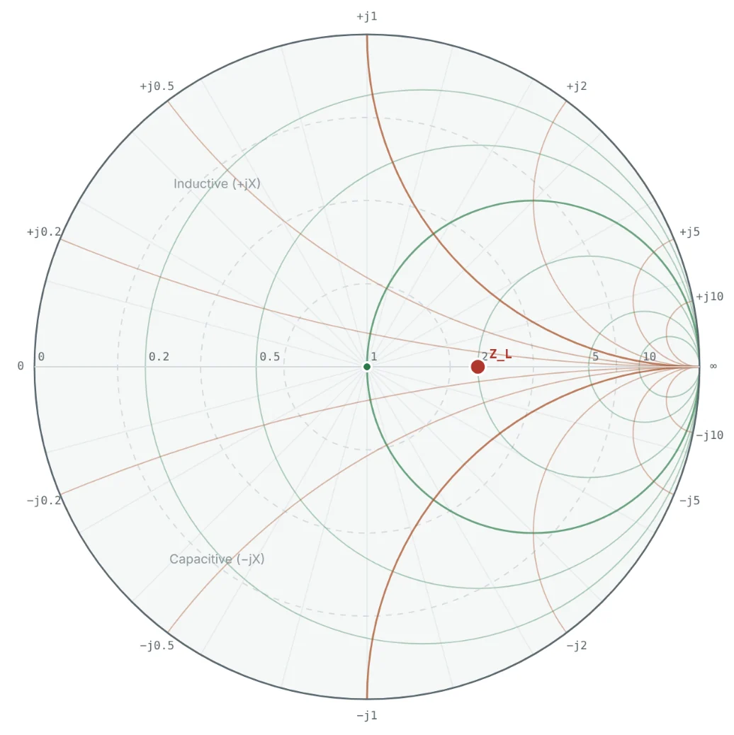
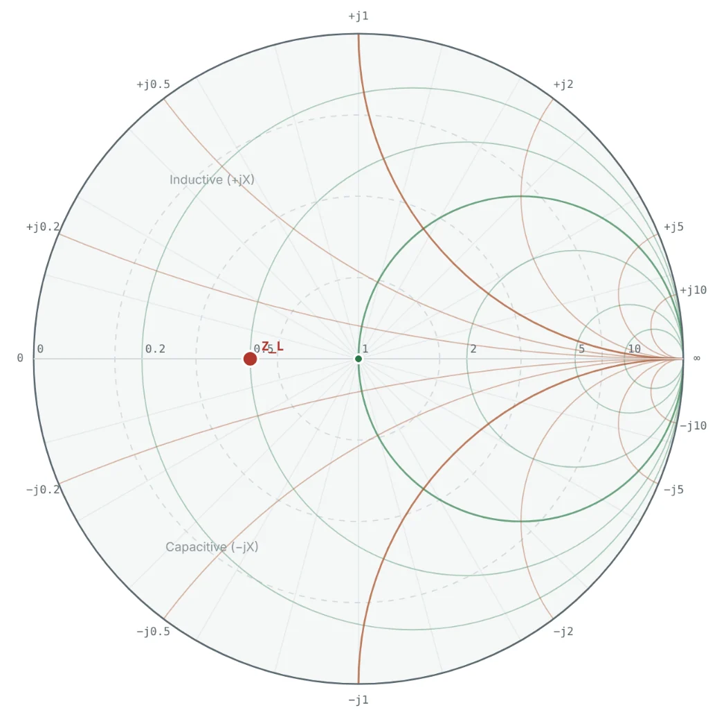
The Smith Chart Calculator computes Γ, S11 and VSWR for any load as you type it. Two loads that are equally mismatched in magnitude but opposite in phase illustrate the geometry well: 100 Ω and 25 Ω on a 50 Ω line both have |Γ| = 1/3, but one is to the right of centre and the other to the left.

Worked Examples
Resistive Loads Above and Below Z₀
Problem: Find Γ for 100 Ω and 25 Ω loads on a 50 Ω line, and the return loss of each.
A load twice Z₀ and a load half Z₀ are equally bad. Mismatch is about the ratio, not the difference.
A Complex Load: 30 − j40 Ω
Problem: Find Γ, the return loss and the reflected power fraction for Z_L = 30 − j40 Ω on a 50 Ω line.
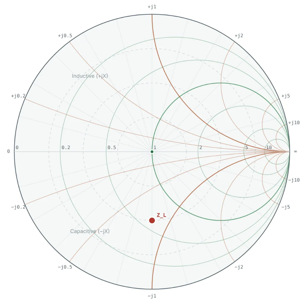

The negative angle confirms the capacitive load. Only 75% of the incident power reaches it.
Inductive Load: 25 + j50 Ω
Problem: A small antenna measures 25 + j50 Ω on a 50 Ω line. What fraction of the power is reflected?
This load is the running example of the series; Part 10 matches it to 50 Ω with two components.
A Purely Reactive Load
Problem: Find Γ for Z_L = j50 Ω on a 50 Ω line.
The point sits at the top of the Smith chart, where the x = +1 arc meets the outer circle.
Recovering the Load From a Measurement
Problem: A network analyser measures S11 = 0.2 ∠ 0° on a 50 Ω port. What is the load?
This is exactly a 75 Ω device on a 50 Ω system — a common, mild mismatch.
Summary
- A load Z_L ≠ Z₀ reflects part of the incident wave; Γ = (Z_L − Z₀)/(Z_L + Z₀) = (z − 1)/(z + 1).
- |Γ| ranges from 0 (matched) to 1 (short, open, or pure reactance); the phase shows whether the load is inductive or capacitive.
- Return loss = −20 log|Γ|; reflected power fraction = |Γ|². The usual target is RL ≥ 10 dB.
- Plotting Γ in the complex plane puts every passive load inside the unit circle — the basis of the Smith chart.
The forward and reflected waves interfere along the line. Part 4: Standing Waves and Voltage Standing Wave Ratio (VSWR) shows the standing-wave pattern they create and how VSWR measures it.
Put It Into Practice
Use the NEXT ANTENNAS calculators to apply the ideas from this article to real designs.