Twelve articles that take you from what impedance is to matching a real antenna — reflection coefficient, VSWR, line transformation, every circle on the Smith chart, and L-network and stub matching, with calculator screenshots and worked examples in every part.
The whole series rests on these four relationships. Each card links to the article that develops it.
Any load can be described by how much of a wave it reflects. Plotting Γ gives the chart.
Part 3 → 2 · VSWR (1 + |Γ|)/(1 − |Γ|)The size of the mismatch: a circle around the centre of the chart.
Part 4 → 3 · Line transformation Γ_in = Γ_L e^(−j2βℓ)Adding line rotates the impedance clockwise; half a wavelength is a full turn.
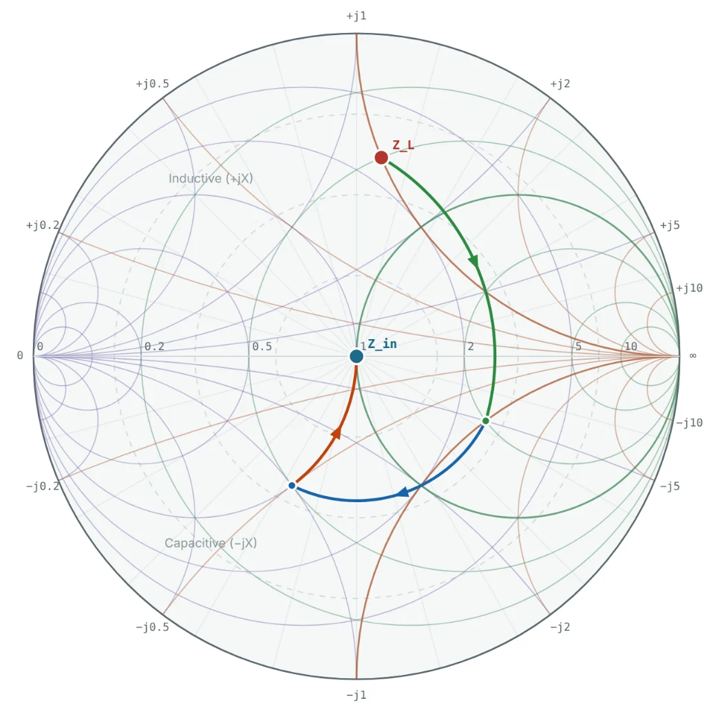
Part 5 → 4 · Matching r circle → g circle → 1Series parts move along resistance circles, shunt parts along conductance circles — to the centre.
Parts 10–11 →Each article builds on the one before it. Read them in order, or jump to the stage you need.
Impedance, characteristic impedance and the reflection coefficient.
What impedance is, how resistance and reactance combine, and why impedance controls power flow at RF.
R + jXReactancePhasorsSeries RLCAdmittanceWhere Z₀ comes from, how to calculate it for coax and microstrip, and why systems use 50 Ω and 75 Ω.
Z₀ = √(L/C)CoaxMicrostrip50 Ω vs 75 Ωε_effWhat happens when a line ends in the wrong load, and how Γ, return loss and S11 measure it.
Γ = (z−1)/(z+1)Return lossS11Short / openReflected powerStanding waves, VSWR and how lines transform impedance.
How forward and reflected waves form standing waves, and how VSWR relates to Γ and mismatch loss.
Standing wavesVSWRV_max / V_minMismatch lossVSWR circleHow a length of line changes impedance: λ/8, λ/4 and λ/2 lines, quarter-wave transformers and stubs.
Z_in equationλ/4 transformerλ/2 lineStubsRotationHow the chart is built, normalised and read.
How the Smith chart is built from the Γ plane, what its regions mean and how impedance and admittance share it.
Γ planeConstructionSpecial pointsAdmittance chartZ/Y chartNormalising and denormalising impedance and admittance, changing Z₀, and turning chart values into parts.
z = Z/Z₀y = Y·Z₀50 vs 75 ΩDenormaliseL and C valuesEvery family of circles on the chart — r, x, g, b, VSWR and constant-Q — and the wavelength scales.
r circlesx arcsg and b circlesWTG scaleConstant QPlotting, lumped and stub matching, and real measurements.
A step-by-step method for plotting any impedance and reading Γ, VSWR, admittance and line transformations.
PlottingReading ΓVSWR circleAdmittanceLine rotationDesign L-networks on the chart: movement rules, four solutions for one load, component values and bandwidth.
Conjugate matchL-networkMovement rulesQ and bandwidthπ / T networksMatch with transmission lines alone: single-stub and double-stub tuners, stub lengths and the forbidden region.
Single stubDouble stubShort vs openMicrostrip lengthsForbidden regionMatching a measured antenna, reading VNA sweeps, lossy-cable spirals, port extension and amplifier circles.
S1P filesVNA sweepsCable lossPort extensionAmplifier circlesThe screenshots in this series were made with the free NEXT ANTENNAS Smith Chart Calculator. Enter the same numbers and you will see the same picture.
A Smith chart is a plot of the reflection coefficient Γ in the complex plane, overlaid with circles of constant resistance and reactance. Every passive impedance maps to a point inside the unit circle, which lets engineers read reflection, VSWR and admittance and design matching networks graphically.
Because it shows impedance, reflection coefficient and the effect of adding components or line length in one picture. Every vector network analyser displays S11 on a Smith chart, and antenna, amplifier and filter design tools use it for matching and for stability, gain and noise circles.
Basic algebra and complex numbers (a + jb, magnitude and angle). Parts 1–5 build the impedance and transmission-line background, so no prior RF experience is required.
Yes. Every chart screenshot in the series comes from the free NEXT ANTENNAS Smith Chart Calculator, which plots loads, builds matching ladders with lumped elements and stubs, sweeps frequency and loads Touchstone .s1p files.
In order from Part 1 if you are new to RF. If you already know impedance, Γ and VSWR, start at Part 6 for the Smith chart itself; if you can already read a Smith chart, go straight to matching in Part 10.
Part 1 takes about 15 minutes and needs no prior RF experience.