Why Normalise?
In Part 3 we wrote Γ = (z − 1)/(z + 1) with z = Z_L/Z₀. The reflection coefficient depends only on the ratio of the load to the line impedance: 100 Ω on a 50 Ω line reflects exactly as much as 150 Ω on a 75 Ω line. By plotting the ratio instead of the ohms, a single chart covers every system. The price is one extra step — dividing by Z₀ before plotting and multiplying by Z₀ after reading.
The centre of every Smith chart is z = 1: "equal to the reference". The grid lines are labelled 0.2, 0.5, 1, 2, 5 — pure numbers, not ohms.
Normalising Impedance and Admittance
| Quantity | Symbol | Normalise | Denormalise | Example (Z₀ = 50 Ω) |
|---|---|---|---|---|
| Resistance | r | R / Z₀ | r · Z₀ | 25 Ω → 0.5 |
| Reactance | x | X / Z₀ | x · Z₀ | +50 Ω → +1 |
| Conductance | g | G · Z₀ | g / Z₀ | 8 mS → 0.4 |
| Susceptance | b | B · Z₀ | b / Z₀ | −16 mS → −0.8 |
A common slip is to divide an admittance by Z₀. Since y = Y/Y₀ and Y₀ = 1/Z₀, normalising an admittance means multiplying it by Z₀. A quick check: the matched admittance Y = 20 mS must give y = 1 on a 50 Ω chart.
Changing the Reference Impedance
Because the chart plots Z/Z₀, the same load moves when the reference changes. Matching to a 75 Ω system means the target is the centre of a 75 Ω chart, which is a different physical impedance from the centre of a 50 Ω chart. In the Smith Chart Calculator the reference is the Z₀ field; change it and every point re-normalises.
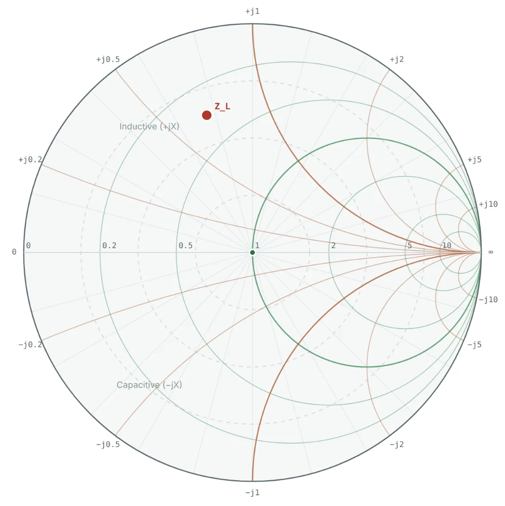

Note that the same load is slightly worse in a 75 Ω system (VSWR 4.44 vs 4.27) — its 25 Ω resistance is further below 75 than below 50, which outweighs the smaller normalised reactance.
From Normalised Values to Components
After a matching design on the chart (Parts 10 and 11), the result is a set of normalised reactances and susceptances. Turning them into parts is a two-step process: denormalise, then divide by ω.
Worked Examples
Normalising to 50 Ω
Problem: Normalise Z = 25 + j50 Ω to Z₀ = 50 Ω and find Γ and VSWR.
The Same Load in a 75 Ω System
Problem: Repeat Example 1 with Z₀ = 75 Ω.
Normalising an Admittance
Problem: The load in Example 1 has admittance Y = 8 − j16 mS. Find y on a 50 Ω chart and check it equals 1/z.
On the chart, y sits diametrically opposite z — the 180° rotation explained in Part 6.
Denormalising a Chart Reading
Problem: A point reads z = 1.2 − j0.6. What impedance is it in a 50 Ω system and in a 75 Ω system?
The chart reading alone is meaningless until you know which Z₀ it was normalised to — always note the reference on a printed chart.
From Normalised Values to Components
Problem: A 900 MHz matching design on a 50 Ω chart calls for a series reactance x = +0.8 and a shunt susceptance b = +1.2. Find the component values.
Summary
- Normalise impedance by dividing by Z₀ (z = r + jx); normalise admittance by multiplying by Z₀ (y = g + jb).
- The chart centre z = 1 always means "equal to the reference impedance".
- Changing Z₀ moves the point and changes Γ and VSWR, but not the physical impedance.
- Denormalise, then divide by ω, to turn chart values into inductors and capacitors.
Part 8: Understanding Smith Chart Parameters and Circles looks closely at the circles and scales on the chart — and the extra ones like constant-Q curves.
Put It Into Practice
Use the NEXT ANTENNAS calculators to apply the ideas from this article to real designs.