Why Match With Stubs?
The L-networks of Part 10 use discrete inductors and capacitors. Above a few gigahertz, their parasitics, tolerances and self-resonances make them hard to use, and component values become very small (fractions of a picofarad, single nanohenries). A transmission line section, on the other hand, is just copper on a substrate: cheap, repeatable and low-loss. From Part 5 we know two facts that make line-only matching possible:
- a length of line in series rotates the impedance around its VSWR circle;
- a short- or open-circuited stub is a pure reactance whose value is set by its length.
Combine a rotating series line with a shunt stub and you have a matching network with no lumped components at all.
Our transmission line series covers stub resonances, open-end effects, T-junction discontinuities and loss in detail. This article focuses on the matching procedure itself. Open the Transmission Line Theory series →
Single-Stub Shunt Matching
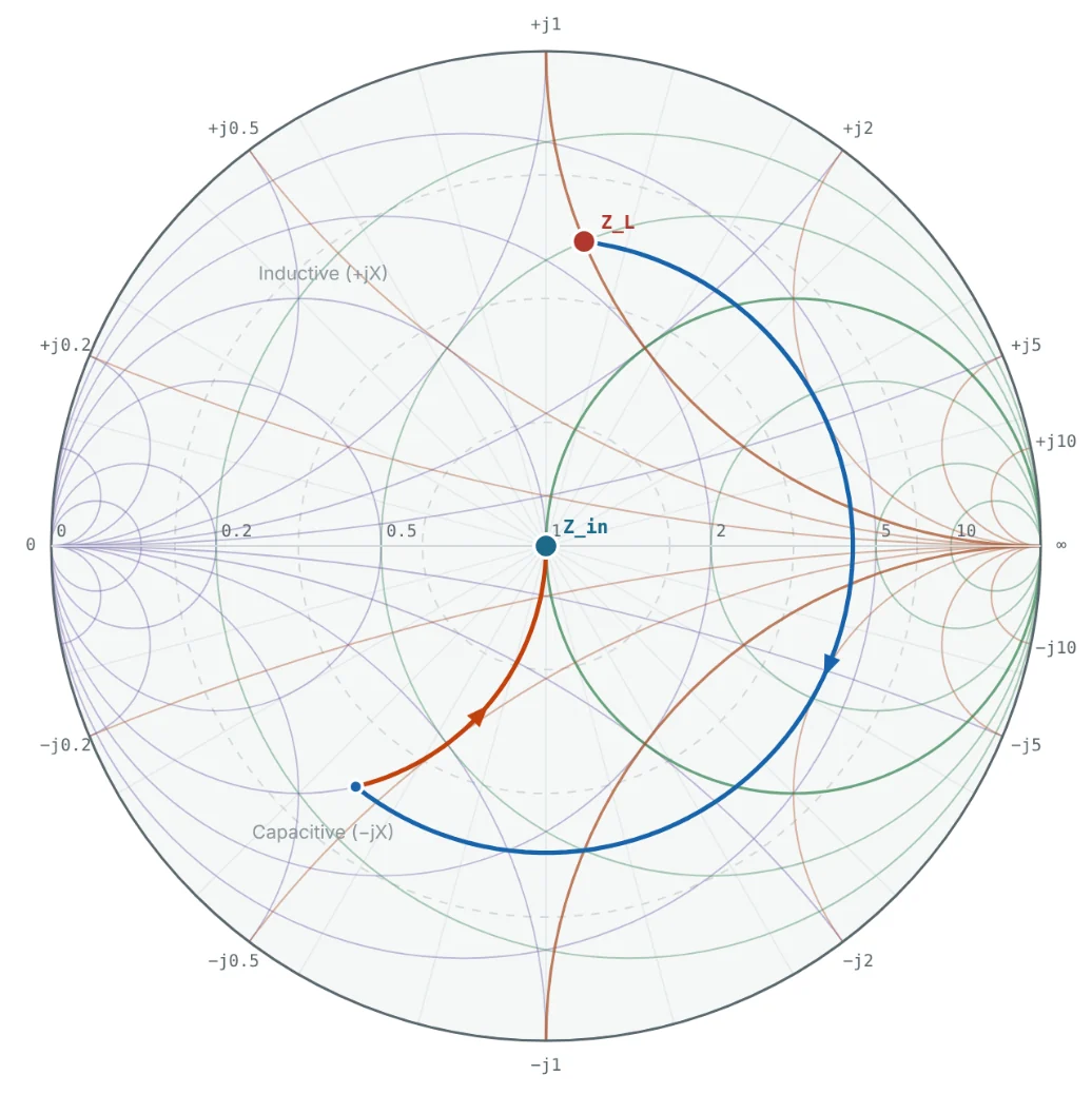
Because the stub is connected in parallel, it adds admittance, so the design is done on the admittance chart (or the combined Z/Y chart):
- Plot the normalised load admittance y_L.
- Rotate clockwise ("toward generator") along the VSWR circle until the point hits the g = 1 circle. There are two intersections, y = 1 + jb and y = 1 − jb. The rotation angle gives d.
- Choose a stub whose susceptance is −jb, so that the total admittance at the stub is exactly 1.
- Find the stub length that gives −jb: start at the short-circuit admittance point (y = ∞, the right edge of the Y chart) or the open-circuit point (y = 0) and rotate clockwise around the outer circle until reaching −jb.
Analytic Solution for d and l
The chart gives the answer to two or three digits; for layout you usually want more. For a load Z_L = R_L + jX_L on a line Z₀ (with R_L ≠ Z₀), let t = tan βd:
Short- or Open-Circuited Stub?
| Consideration | Short-circuited stub | Open-circuited stub |
|---|---|---|
| Construction (coax, waveguide) | Preferred: a short is easy to make and does not radiate | An open end radiates and has fringing capacitance |
| Construction (microstrip) | Needs a via to ground, which adds inductance | Preferred: no via; correct for the open-end extension |
| DC behaviour | Shorts the line at DC (can provide a bias return) | Transparent at DC |
| Length for inductive b (b < 0) | < λ/4 | > λ/4 |
| Length for capacitive b (b > 0) | > λ/4 | < λ/4 |
Shorter stubs are usually better: they occupy less space and are less frequency-sensitive, giving a wider bandwidth.
Double-Stub Tuning
A single-stub tuner needs the stub at a specific position d, which changes with every load. That is fine on a PCB, but awkward in a coaxial or waveguide tuner where the stub position is fixed by the mechanics. A double-stub tuner uses two stubs at fixed positions, separated by a fixed spacing (commonly λ/8, 3λ/8 or λ/4), and achieves a match by adjusting only the two stub lengths.
The design works backwards from the matched point:
- At stub 2 the admittance must be on the g = 1 circle (so stub 2 can cancel the susceptance).
- Moving back toward the load by d rotates the g = 1 circle counter-clockwise by 720° × d/λ. This rotated g = 1 circle is where the admittance must be just after stub 1.
- Stub 1 moves the load admittance along its constant-g circle until it meets the rotated circle.
- Rotate that point clockwise by d (it lands on g = 1), then choose stub 2 to cancel the remaining susceptance.
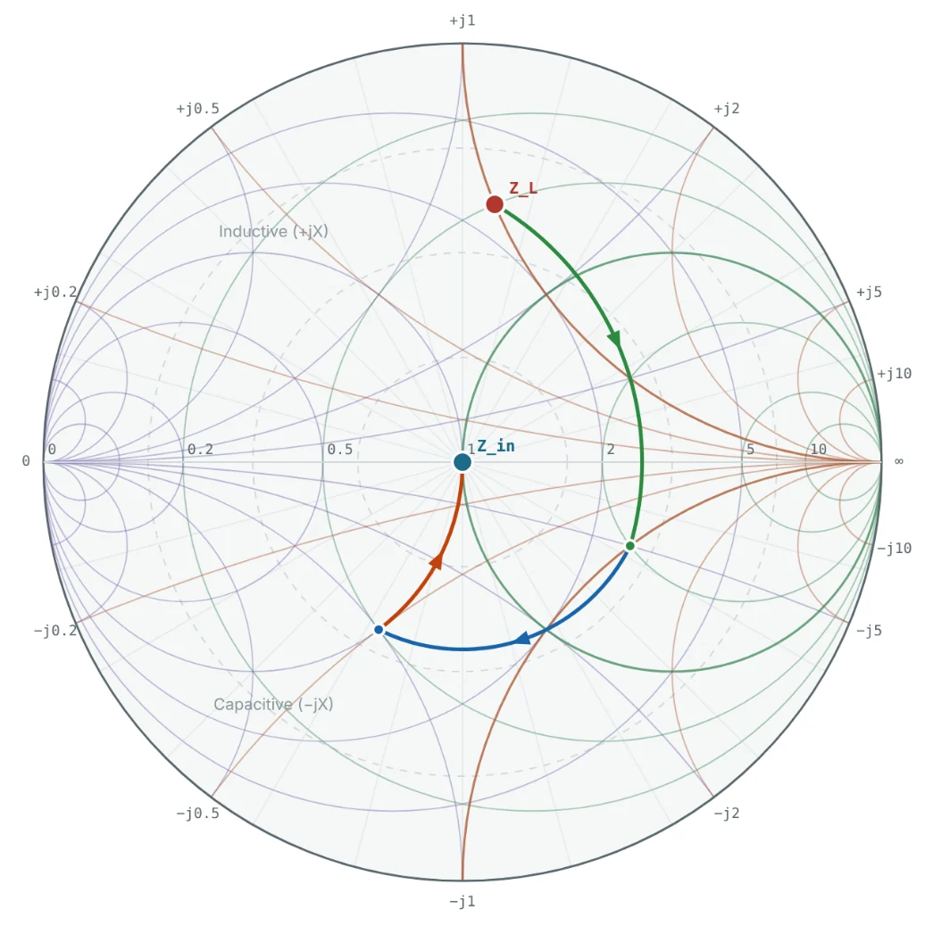
Stub 1 can only move along the load's constant-g circle. If that circle never touches the rotated g = 1 circle, no match exists. For stub spacing d the forbidden region is g > 1/sin²(βd): for λ/8 spacing, any load with g > 2. Moving the tuner a short distance along the line (λ/8, say) changes y_L and usually escapes the region.

Bandwidth of Stub Matching
Every line section in a stub tuner has an electrical length proportional to frequency, so the match degrades faster than with lumped elements. For the same 25 + j50 Ω load at 2.4 GHz, the shortest single-stub solution gives:
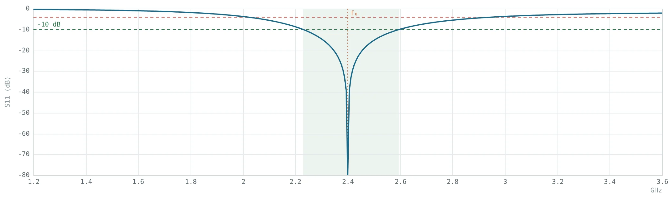

To widen the band, use the solution with the shortest d and l, keep stubs close to the load, use lower-impedance (wider) stubs, or use two stubs in parallel (a "balanced" stub on each side of the line) — which also reduces the stub length needed.
Worked Examples
Single-Stub Match: Solution 1
Problem: Design a short-circuited shunt stub to match 25 + j50 Ω to 50 Ω. Use the solution closest to the load.
At d₁ the admittance is y = 1 + j1.581, so the stub must supply b_s = −1.581 (inductive): l = arccot(1.581)/2π = 0.0898 λ.

Single-Stub Match: Solution 2
Problem: Find the second solution and the shorter of its two stub options.
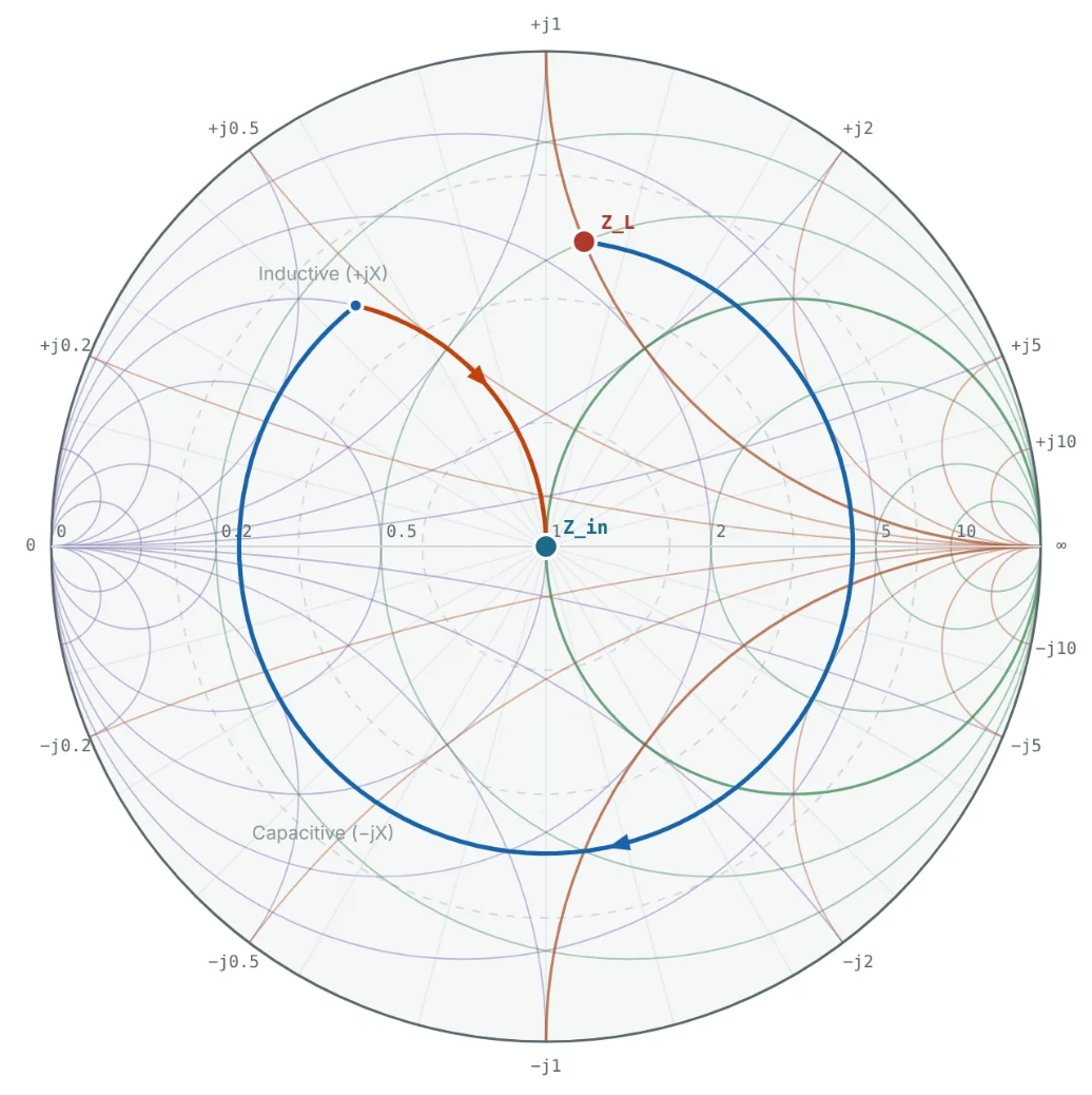
A capacitive susceptance is shortest as an open stub. Solution 1 is still preferable because both its line and stub are shorter.
Physical Lengths on FR-4
Problem: Convert both solutions to millimetres for 50 Ω microstrip on 1.6 mm FR-4 at 2.4 GHz (ε_eff = 3.32, λ_g = 68.56 mm).
| Solution | d | Short stub | Open stub |
|---|---|---|---|
| 1 | 0.2933 λ = 20.11 mm | 0.0898 λ = 6.15 mm | 0.3398 λ = 23.29 mm |
| 2 | 0.4369 λ = 29.95 mm | 0.4103 λ = 28.13 mm | 0.1603 λ = 10.99 mm |
In practice, shorten an open stub by the open-end extension (≈ 0.6 mm here) and account for the via inductance of a shorted stub. The Microstrip Calculator gives λ_g for other substrates.
Double-Stub Tuner With λ/8 Spacing
Problem: Match y_L = 0.4 − j0.8 with short stubs at the load and λ/8 toward the source.
The alternative intersection needs b₁ = +2.6 (l₁ = 0.4416 λ) and b₂ = +3.0 (l₂ = 0.4488 λ) — longer stubs and a narrower band, so the first solution is preferred.
A Load in the Forbidden Region
Problem: Can the same λ/8-spaced tuner match a 10 Ω resistive load?
Adding λ/8 of 50 Ω line between the load and the tuner rotates y_L = 5 to y = 0.385 − j0.923 (g < 2), after which the tuner can match it.
Summary
- Single-stub matching rotates the load along its VSWR circle to g = 1, then a shunt stub cancels the susceptance; there are two solutions per load.
- Stub length follows from y = −j cot βl (short) or +j tan βl (open); the two differ by λ/4.
- Double-stub tuners have fixed positions and adjustable lengths but cannot match loads with g > 1/sin²(βd).
- Stub matches are narrower-band than lumped L-networks; choose the shortest line and stub lengths.
Part 12: Practical Applications of Smith Charts in RF and Microwave Engineering closes the series by applying everything to real measured devices.
Put It Into Practice
Use the NEXT ANTENNAS calculators to apply the ideas from this article to real designs.