Introduction to Impedance
Ask an RF engineer what an antenna "is" and the first answer will usually be a number like "about 50 ohms at 2.4 GHz". Ask what is wrong with a poorly performing amplifier and the answer is often "it's mismatched". Both answers are about impedance. Impedance tells us how a circuit resists and stores energy when an alternating current flows through it, and at radio frequencies almost every design decision — line widths, connector choices, component values, antenna dimensions — is made to control it.
This twelve-part series builds from that idea to the Smith chart, the graphical tool engineers use to visualise and manipulate impedance. This first part covers the foundation: what impedance is, how it is written, and how it behaves with frequency.
What Is Electrical Impedance?
Impedance (Z) is the ratio of the voltage across a component to the current through it, for a sinusoidal signal. It extends Ohm's law from DC to AC: it tells us not only how large the current is for a given voltage, but also how much the current is shifted in time relative to the voltage.
Impedance has two parts with very different physical meanings. The resistance R represents energy that leaves the circuit — dissipated as heat in a resistor or radiated as electromagnetic waves by an antenna. The reactance X represents energy that is stored and returned every cycle, in the magnetic field of an inductor or the electric field of a capacitor.
Resistance, Inductance, and Capacitance
| Element | Impedance | Phase of V vs I | Frequency behaviour | Energy |
|---|---|---|---|---|
| Resistor R | Z_R = R | In phase (0°) | Constant (ideally) | Dissipated |
| Inductor L | Z_L = jωL | V leads I by 90° | Rises with f | Stored in magnetic field |
| Capacitor C | Z_C = 1/(jωC) = −j/(ωC) | V lags I by 90° | Falls with f | Stored in electric field |
Here ω = 2πf is the angular frequency in rad/s. A useful memory aid is "ELI the ICE man": in an inductor (L) the voltage (E) leads the current (I); in a capacitor (C) the current (I) leads the voltage (E).
At RF, real components are never pure. A chip resistor has a little series inductance and shunt capacitance; a capacitor has series inductance from its leads and pads, which makes it self-resonate and behave like an inductor above that frequency; an inductor has winding capacitance. These "parasitics" are why datasheets give S-parameters and why the Smith chart, which shows the true impedance at each frequency, is so useful.
Real and Imaginary Components of Impedance
Because resistance and reactance act 90° apart, they cannot simply be added as ordinary numbers. Impedance is written as a complex number, with resistance as the real part and reactance as the imaginary part:
The reciprocal of impedance is admittance, Y = 1/Z = G + jB, measured in siemens. G is the conductance and B the susceptance. Admittance is more convenient whenever components are connected in parallel, because parallel admittances simply add — a fact the Smith chart exploits for shunt matching components in Part 8 and Part 10.
Complex Impedance and Phasor Representation
A sinusoidal voltage v(t) = V_m cos(ωt + φ) can be represented by a phasor — a complex number V = V_m e^{jφ} that keeps the amplitude and phase and drops the time variation. With phasors, differentiation becomes multiplication by jω, so the differential equations of AC circuits become simple algebra. Impedance is then just the ratio of two phasors, and it can be written in two equivalent ways:
Inductive and Capacitive Impedance
Impedance in AC Circuits
Impedances combine exactly like resistances: in series they add, in parallel their admittances add. For a series R, L and C:
Resonance is everywhere in RF: an antenna is designed to be resonant (purely resistive) at its operating frequency, filters are built from resonators, and a matching network works by adding just enough reactance of the opposite sign to cancel a load's reactance.
Importance of Impedance in RF Engineering
Worked Examples
Reactance of a 10 nH Inductor
Problem: Find the reactance of a 10 nH chip inductor at 100 MHz and at 2.4 GHz.
The same part is almost a short circuit at 100 MHz and a large impedance at 2.4 GHz. This is why RF chokes (inductors that block RF but pass DC bias) work, and why a few millimetres of PCB trace (roughly 1 nH per mm) matters at microwave frequencies.
Reactance of a 1 pF Capacitor
Problem: Find the reactance of a 1 pF capacitor at 2.4 GHz.
A DC-blocking capacitor at 2.4 GHz should have a reactance of only a few ohms, so values of 10–100 pF are used. A 1 pF capacitor is instead a typical matching component.
Series RLC Impedance and Resonance
Problem: A 50 Ω resistor, the 10 nH inductor and the 1 pF capacitor are connected in series. Find Z at 2.4 GHz in rectangular and polar form, and the resonant frequency.
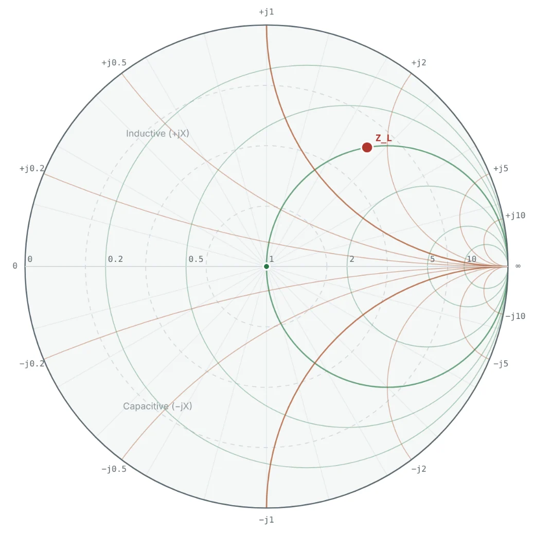
Above resonance the inductor dominates, so the circuit is inductive. At 1.59 GHz the reactances cancel and Z = 50 Ω exactly — a perfect match to a 50 Ω system.
Polar to Rectangular — and the Component Behind It
Problem: An impedance analyser shows Z = 100 ∠ −30° Ω at 1 GHz. Convert it to rectangular form and find the series component that represents the reactance.
A negative angle always means capacitive. The equivalent capacitance is only valid at 1 GHz; at another frequency the same physical device would show a different angle.
Parallel RC to Series Form
Problem: A 100 Ω resistor in parallel with 1 pF models a device input at 1 GHz. What is the equivalent series impedance?
The parallel capacitor lowers both the resistance and the reactance seen in series form. Converting between series and parallel forms — or between impedance and admittance — is exactly what the Smith chart does graphically by a 180° rotation (Part 8).
Summary
| Quantity | Expression | Remember |
|---|---|---|
| Impedance | Z = V/I = R + jX | Ohm's law for AC, in ohms |
| Polar form | |Z| = √(R² + X²), θ = tan⁻¹(X/R) | Magnitude and phase |
| Inductor | X_L = +2πfL | Positive, rises with f |
| Capacitor | X_C = −1/(2πfC) | Negative, falls with f |
| Admittance | Y = 1/Z = G + jB | Parallel admittances add |
| Series resonance | f₀ = 1/(2π√(LC)) | Reactances cancel, Z = R |
- Impedance combines resistance (energy lost or radiated) and reactance (energy stored) into one complex number.
- Inductive reactance is positive and grows with frequency; capacitive reactance is negative and shrinks with frequency.
- Rectangular form adds easily; polar form shows magnitude and phase; admittance makes parallel circuits easy.
- Almost every RF design goal — power transfer, low reflection, gain, bandwidth — is an impedance goal.
Next, Part 2: Understanding Characteristic Impedance of Transmission Lines introduces the impedance that a transmission line itself presents, and why RF systems standardise on 50 Ω and 75 Ω.
Put It Into Practice
Use the NEXT ANTENNAS calculators to apply the ideas from this article to real designs.