Why Transmission Line Theory?
In a first course on circuits, every wire is assumed to be ideal — zero resistance, zero inductance, zero propagation delay. Voltages and currents exist uniformly throughout the circuit at every instant. This is the lumped-circuit model, and it is extraordinarily useful at power frequencies (50/60 Hz) and audio frequencies.
At radio frequencies this model fails — not because the physics changes, but because the wavelength of the signal becomes comparable to the physical size of the conductors and components. When that happens, voltage and current are no longer uniform along a conductor. They vary with position. The wire itself becomes a distributed element, and the simple V = IR model is no longer enough.
Transmission line theory is the branch of electromagnetics that describes how signals propagate along conductors when the lumped-circuit approximation no longer holds. It sits between basic circuit theory and full Maxwell's equations — it is more accurate than lumped circuits, and far more tractable than solving the full 3D EM problem from scratch. Every RF and microwave engineer uses it daily.
A 1 GHz signal has a free-space wavelength of 30 cm. A PCB trace connecting a transmitter IC to an antenna connector might be 3 cm long — that is λ/10. At this scale, the voltage at one end of the trace can be significantly different from the voltage at the other end at the same instant in time. The lumped model — which assumes they are the same — introduces serious errors.
What Goes Wrong with Lumped Circuits?
The lumped approximation is valid when the physical dimensions of the circuit are much smaller than the wavelength of the signal. When the size becomes comparable to the wavelength, three things happen that the lumped model cannot predict:
- Propagation delay becomes significant. It takes time for a signal to travel along a conductor. At 1 GHz the propagation time along a 15 cm trace is comparable to half a period — signals at the two ends of the trace are out of phase.
- Standing waves appear. When the load impedance does not match the source, signals reflect back toward the source. The incident and reflected waves superimpose to form a standing wave pattern along the line — with voltage maxima and minima distributed along its length. Lumped circuits cannot model this.
- Impedance depends on position. The impedance seen looking into a transmission line changes with the electrical length of the line. A short circuit 90° away looks like an open circuit. An open circuit 90° away looks like a short circuit. This is completely invisible to lumped circuit analysis.
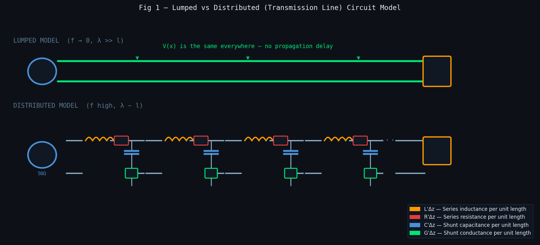
In the distributed model the line is divided into infinitesimally small sections, each with a series inductance L'Δz, series resistance R'Δz, shunt capacitance C'Δz, and shunt conductance G'Δz. Applying Kirchhoff's laws to each section and taking the limit as Δz → 0 yields the telegrapher's equations — the coupled partial differential equations that govern voltage and current on a transmission line:
When Must a Line Be Treated as a Transmission Line?
The practical question every RF engineer must answer is: at what point does my conductor stop behaving like a simple wire and start needing a transmission line treatment? The answer is based on the ratio of the physical length of the conductor to the signal wavelength — the electrical length.
The commonly used rule of thumb is:
- l < λ/10 (θe < 36°): Lumped circuit analysis is acceptable. Transmission line effects are small and can usually be ignored in most engineering applications.
- λ/10 ≤ l < λ/4 (36° ≤ θe < 90°): Transmission line effects are significant and must be accounted for. Lumped circuit analysis gives incorrect results.
- l ≥ λ/4 (θe ≥ 90°): Full transmission line analysis is essential. Impedance transformation, reflections, and standing waves are dominant design considerations.
Consider a 5 cm microstrip trace on FR-4 (εeff ≈ 3.5). At what frequency must it be treated as a transmission line?
The guided wavelength is λeff = c/(f·√εeff). The λ/10 limit gives: l = λeff/10 → f = c/(10·l·√εeff) = 3×10⁸/(10 × 0.05 × √3.5) = 3×10⁸/0.296 ≈ 1.01 GHz.
Below ~1 GHz, this trace can be treated as a lumped element. Above 1 GHz, it must be designed and analysed as a transmission line — accounting for its characteristic impedance, reflections from impedance discontinuities, and its effect on the signal phase.
Other situations that always require transmission line treatment, regardless of frequency:
- Any cable connecting a transmitter to an antenna — even at HF (3–30 MHz), a 10 m coaxial cable is electrically long
- Interconnects inside RF modules and microwave ICs
- PCB traces in any design operating above 500 MHz
- Waveguide runs in radar, satellite, and mmWave systems
- Any structure where impedance matching between source and load matters
Types of Transmission Lines
Transmission lines come in many physical forms, each with different geometries, field distributions, frequency ranges, and applications. All of them share the same theoretical foundation — the telegrapher's equations — but differ in their characteristic impedance, loss, dispersion, and how they confine the electromagnetic field.
Two-Wire Line
The two-wire line — also called a parallel-wire line or balanced line — is the simplest transmission line geometry: two parallel conducting wires separated by a dielectric spacer or air. It is the structure that gives rise to the telegrapher's equations in their most basic form.
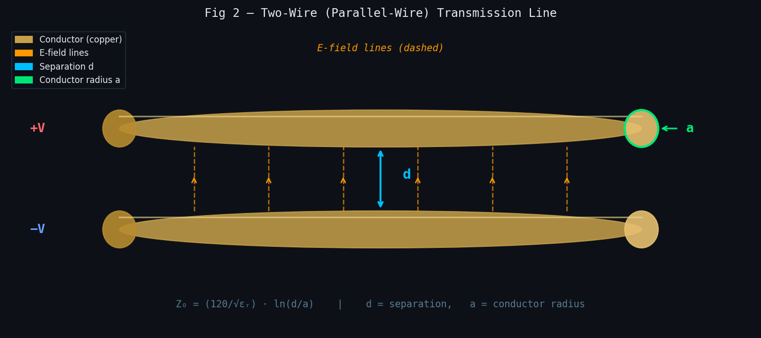
Two-wire lines support a TEM (transverse electromagnetic) mode — both the electric and magnetic fields are entirely perpendicular to the direction of propagation. This means they can operate from DC to the frequency at which higher-order modes begin to propagate. Common examples include 300 Ω ribbon cable for TV aerials and ladder-line for amateur radio antenna feeders. Their main disadvantage is that they radiate — the fields extend into the surrounding space — making them unsuitable for dense circuits or shielded environments.
Coaxial Cable
The coaxial cable solves the radiation problem of the two-wire line by enclosing the inner conductor within a coaxial outer conductor (shield). All electromagnetic fields are confined between the two conductors — no energy radiates outward, and external interference is rejected. This is the most widely used transmission line for connecting RF equipment.
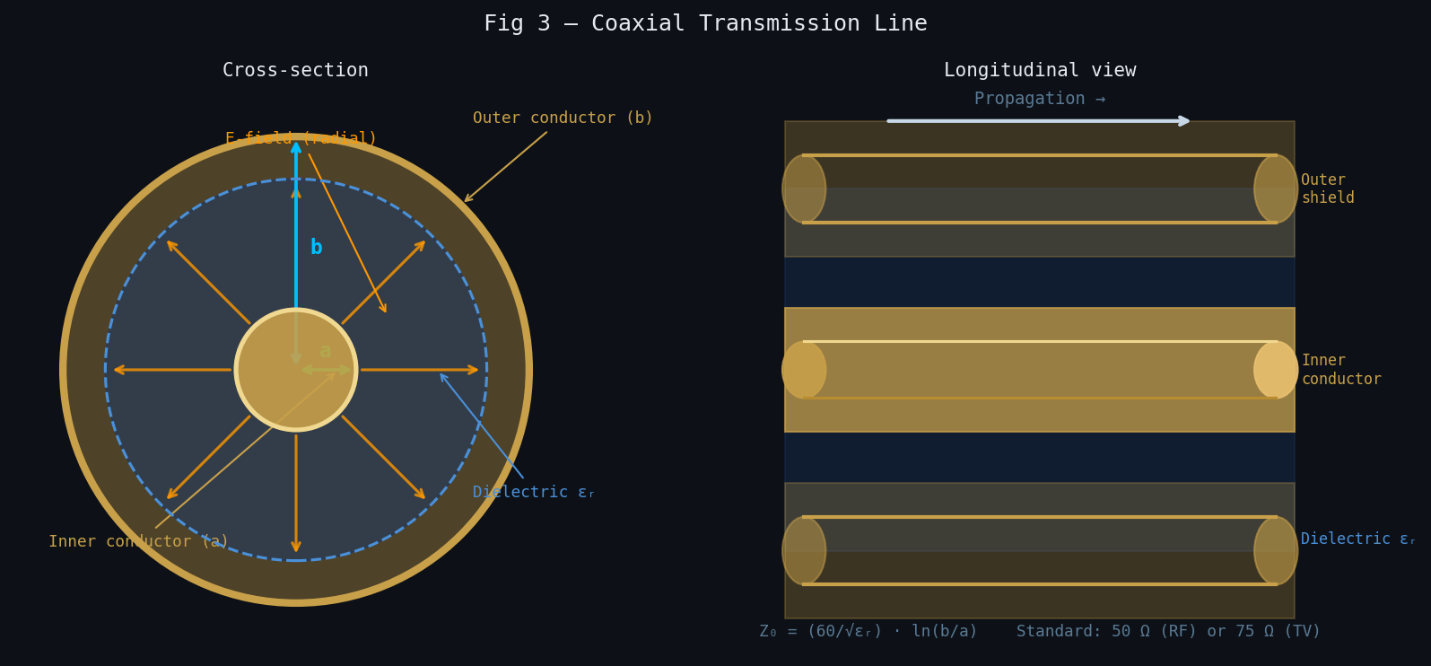
Standard coaxial impedances are 50 Ω (most RF/microwave work) and 75 Ω (cable television and video). The 50 Ω standard is a practical compromise between minimum loss (~77 Ω for air-filled coax) and maximum power handling (~30 Ω). Like two-wire lines, coaxial cable supports a TEM mode from DC up to the frequency at which the first higher-order TE or TM mode can propagate.
Planar Transmission Lines
Planar transmission lines are fabricated using printed circuit board (PCB) processes — the conductors are etched onto the surface of a dielectric substrate. They are the dominant technology in RF and microwave integrated circuits, PCB-level RF design, and monolithic microwave integrated circuits (MMICs). The three most important types are microstrip, stripline, and coplanar waveguide.
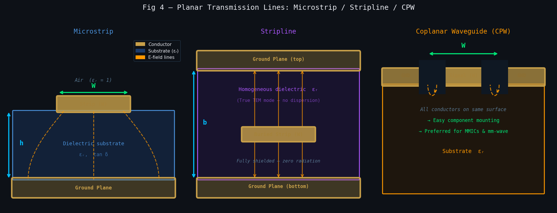
Microstrip — the most widely used planar line. The signal conductor sits on the top surface of the substrate; the ground plane is on the bottom. Part of the field travels through the substrate, part through the air above — giving a mixed-medium effective permittivity εeff between 1 and εr. This makes microstrip slightly dispersive (phase velocity varies with frequency) and gives it a quasi-TEM mode rather than a true TEM mode. It is easy to fabricate, easy to solder components to, and allows integration with active devices.
Stripline — the strip conductor is buried between two ground planes inside the substrate. The field is entirely contained within the homogeneous dielectric — stripline supports a true TEM mode with no dispersion. It is completely shielded from radiation and external interference. The disadvantage is that it is harder to access for component mounting and the structure is more expensive to fabricate. Used in multilayer PCBs when shielding and low dispersion are required.
Coplanar Waveguide (CPW) — the signal conductor and both ground conductors are on the same surface, separated by gaps. This puts all conductors in one plane, making it very easy to connect surface-mount components without vias. CPW supports a quasi-TEM mode. It is the preferred structure for MMIC (monolithic microwave integrated circuit) design at mm-wave frequencies because the ground reference is immediately adjacent to the signal trace.
Waveguides
A metallic waveguide is a hollow conducting tube — rectangular or circular in cross-section — through which electromagnetic waves propagate. Unlike the TEM-mode lines above, waveguides support TE (transverse electric) or TM (transverse magnetic) modes, not TEM. This has a critical consequence: waveguides have a cutoff frequency below which they cannot propagate any signal.
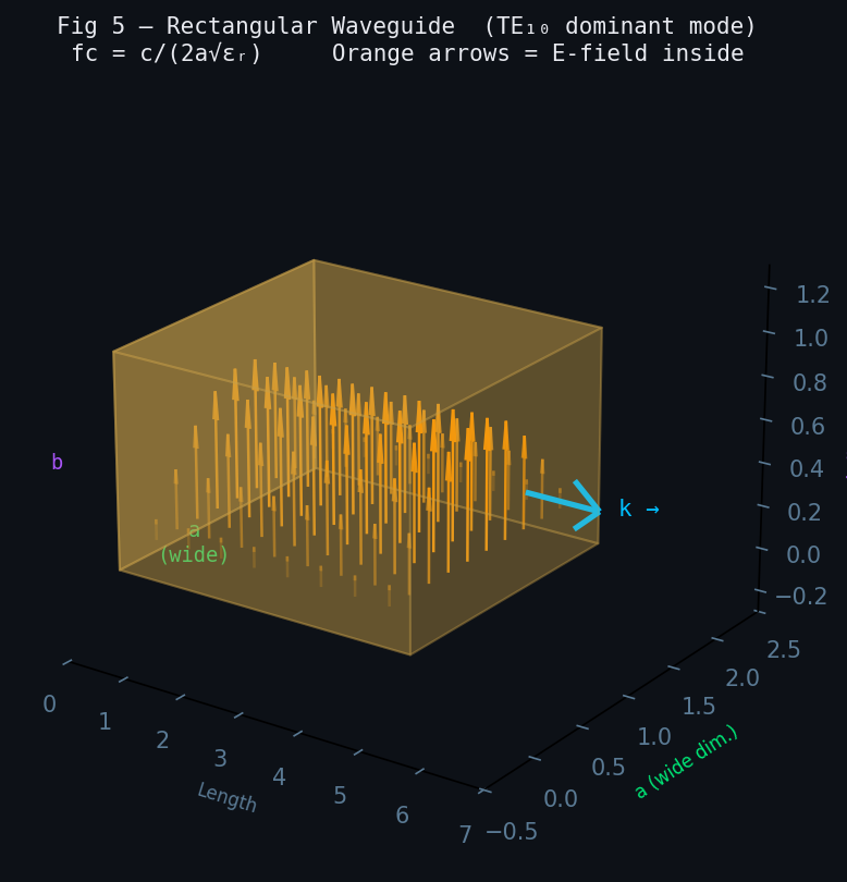
Waveguides have very low loss at microwave and mm-wave frequencies — far lower than coaxial cable — and can handle very high power levels. This makes them the preferred transmission medium for radar transmitters, satellite earth station feeds, and high-power accelerator systems. Their main disadvantages are physical bulk, the need for precision machining, and the fact that they cannot operate below their cutoff frequency.
The table below summarises the key properties of the four main transmission line families:
| Type | Mode | Shielded? | Typical Z₀ | Frequency range | Main use |
|---|---|---|---|---|---|
| Two-wire | TEM | No | 100–600 Ω | DC – VHF | Balanced antenna feeders |
| Coaxial | TEM | Yes | 50 Ω / 75 Ω | DC – 50 GHz | RF cables, connectors |
| Microstrip | quasi-TEM | Partial | 20–120 Ω | DC – 100 GHz | PCB RF design, filters |
| Stripline | TEM | Yes | 20–120 Ω | DC – 40 GHz | Multilayer PCB, shielded |
| CPW | quasi-TEM | Partial | 20–120 Ω | DC – 200 GHz | MMICs, mm-wave |
| Waveguide | TE / TM | Yes | – | f > f_c only | Radar, satellite, high power |
Movement of a Signal Along a Transmission Line
When a source applies a voltage to the input of a transmission line, the signal does not arrive instantaneously at the load. It travels as an electromagnetic wave guided by the conductors, at a velocity determined by the properties of the medium between the conductors. This is the phase velocity:
The propagation constant γ describes how the wave changes as it travels along the line. For the general (lossy) case it has a real part α (attenuation constant) and an imaginary part β (phase constant):
Incident and Reflected Waves
The general solution to the telegrapher's equations gives two travelling wave components — one travelling in the +z direction (toward the load) and one in the −z direction (back toward the source):
When the wave reaches the load, what happens depends entirely on whether the load impedance matches the characteristic impedance of the line. Three key cases:
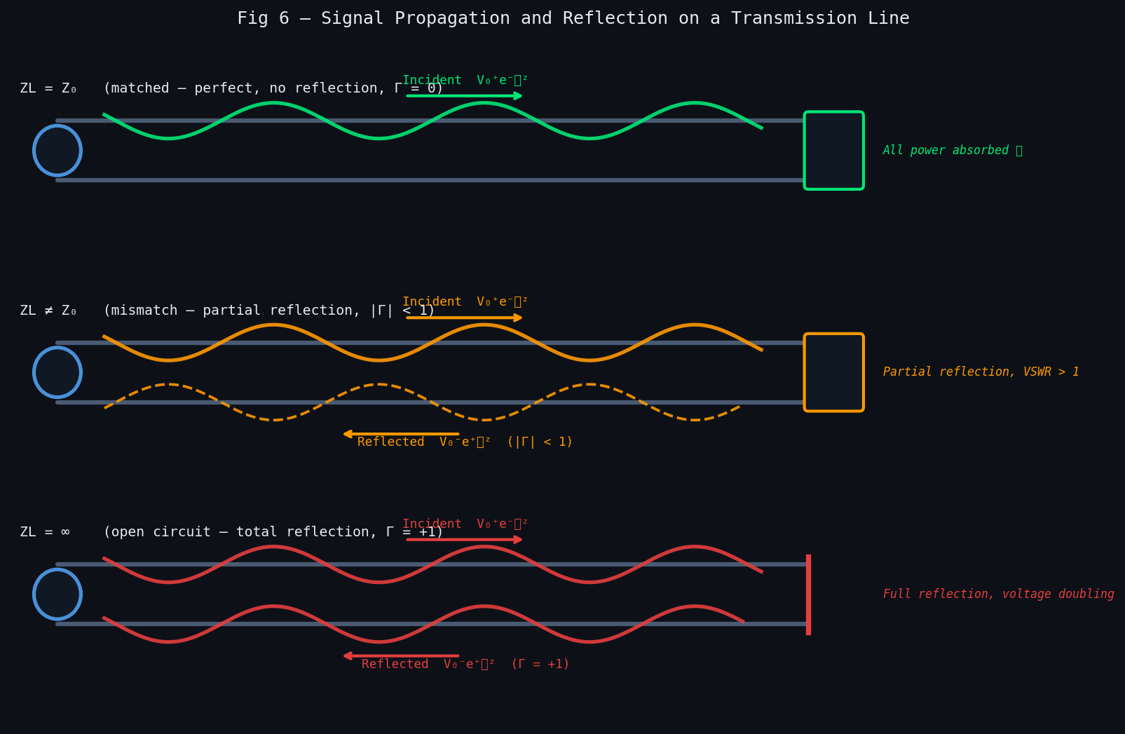
- Z_L = Z₀ (matched): The reflection coefficient Γ = 0. The incident wave is fully absorbed by the load. No reflected wave exists. Maximum power transfer. VSWR = 1.
- Z_L ≠ Z₀ (mismatched): A reflected wave travels back toward the source. The reflected wave amplitude is |Γ| times the incident amplitude. The incident and reflected waves interfere to create a standing wave pattern. VSWR > 1.
- Z_L = ∞ (open circuit): Γ = +1. Total reflection with voltage doubling at the open end. VSWR = ∞.
- Z_L = 0 (short circuit): Γ = −1. Total reflection with phase reversal. Current doubles at the short. VSWR = ∞.
Characteristic Impedance Z₀
The characteristic impedance is the single most important parameter of any transmission line. It is defined as the ratio of voltage to current for a wave travelling in one direction on an infinite (or matched) line:
Z₀ is a property of the transmission line geometry and the dielectric material — it is independent of the line's length and of the source or load connected to it. It is set entirely by the per-unit-length inductance L' and capacitance C'. Designing a transmission line means choosing the geometry (width, spacing, substrate) to achieve the desired Z₀ — almost always 50 Ω in RF work.
This article has established why transmission line theory is needed and what a transmission line is. The next articles in this series cover the mathematics in detail — the Telegrapher's equations and their wave solutions, characteristic impedance and how to calculate it for specific line types, the reflection coefficient and VSWR, and the Smith chart as a design tool.
Questions & Worked Examples
Apply the concepts from this article to real engineering problems. Work through each question before checking the solution.
Electrical Length — Is This Trace a Transmission Line?
Problem: A microstrip trace on Rogers RO4003C (εr = 3.55, εeff ≈ 2.9) is 8 cm long. At what frequency does it reach λ/10 electrical length and must be treated as a transmission line? At 5 GHz, what is its electrical length in degrees?
Above 220 MHz this trace must be designed as a transmission line. At 5 GHz it spans more than two full wavelengths — impedance discontinuities, reflections, and standing waves will all be prominent. Proper 50 Ω width control and matched termination are essential.
Two-Wire Line — Characteristic Impedance
Problem: A twin-lead feeder for a 300 MHz FM antenna consists of two copper conductors, each with radius a = 0.5 mm, separated by d = 8 mm (centre-to-centre), in air (εr = 1). Calculate the characteristic impedance Z₀.
This is close to the standard 300 Ω twin-lead used for TV aerials. To achieve exactly 300 Ω with a = 0.5 mm, d = 0.5 × e^(300/120) = 0.5 × e^2.5 = 0.5 × 12.18 ≈ 6.1 mm separation would be needed. The unshielded field of a two-wire line means it both radiates and picks up interference — suitable for antenna feeders but not for board-level RF interconnects.
Coaxial Cable — Impedance from Geometry
Problem: A coaxial cable has an inner conductor radius a = 0.455 mm and a PTFE dielectric (εr = 2.1). What inner radius b of the outer conductor is needed to achieve Z₀ = 50 Ω? What is the phase velocity as a fraction of c?
This matches the geometry of RG-316 coaxial cable (a ≈ 0.46 mm, b ≈ 1.50 mm, PTFE fill, rated 50 Ω). The 69% velocity factor means a 1 m physical length is electrically equivalent to 1.45 m of free-space propagation — critical to account for when designing phase-matched cable assemblies and antenna arrays.
Waveguide Cutoff Frequency
Problem: A WR-90 rectangular waveguide (standard X-band) has inner dimensions a = 22.86 mm (wide) × b = 10.16 mm (narrow), air-filled (εr = 1). Calculate: (a) the TE₁₀ cutoff frequency, (b) the operating frequency range before the next mode TE₂₀ propagates, and (c) the phase velocity at 10 GHz.
The X-band specification (8.2–12.4 GHz) builds in margin well above the 6.56 GHz cutoff and well below the 13.12 GHz second-mode onset. The superluminal phase velocity is a property of guided-wave dispersion — the group velocity at 10 GHz is v_g = c² / v_p = c / 1.325 ≈ 0.755c, confirming that energy (and information) travels slower than light.
Reflection at a Load — Propagation Constant and Reflected Voltage
Problem: A lossless 50 Ω coaxial transmission line is connected to a load Z_L = 75 + j25 Ω at 2.4 GHz. (a) Calculate the reflection coefficient Γ. (b) What fraction of the incident power is reflected? (c) If the incident voltage amplitude is V₀⁺ = 10 V, what is the reflected voltage amplitude?
A VSWR of 1.77:1 and return loss of 11.1 dB is a borderline match — just above the 10 dB (VSWR 2:1) minimum criterion. For a transmitter port this would be acceptable in most applications, but for a receiver LNA input the mismatch degrades noise figure. An L-network or quarter-wave transformer between the 50 Ω line and the 75+j25 Ω load would bring VSWR to 1:1.