Power Consumption
Biasing Techniques
The transistor bias point is the single most consequential decision in LNA design — it determines NF_min, g_m, IIP3, and DC power consumption simultaneously. Three biasing strategies are used in practice:
Fixed Voltage Bias (Resistive Divider)
A resistive voltage divider from VDD sets V_GS directly. Simple, cheap, and process-independent, but sensitive to temperature variation and transistor threshold voltage spread. The bias resistors must be large enough (typically > 10 kΩ) that their contribution to the noise and impedance at the gate is negligible at RF. An RF choke inductor or high-impedance bias line prevents the resistors from loading the RF signal path.
Current Mirror Bias
A reference current I_ref flows through a diode-connected transistor M_ref. The same V_GS is replicated in the LNA transistor M1, which mirrors I_ref scaled by the transistor width ratio W1/W_ref. Current mirror biasing is accurate, process-tracking (both transistors track together over process corners), and temperature-stable when combined with a bandgap reference. It is the dominant biasing approach in integrated LNA designs.
Active Bias / Self-Bias
In discrete LNA MMICs, active bias circuits sense the drain current and adjust the gate voltage via a feedback loop to maintain a stable operating point. This is critical in GaAs and GaN devices where V_th can vary significantly between devices and with temperature. Active bias circuits add a few milliamps of overhead but dramatically improve yield and performance consistency across temperature (−40 to +85°C commercial range, or −55 to +125°C military).
Power vs Noise vs Gain Trade-offs
Increasing the drain bias current I_DS has a complex, non-monotonic effect on LNA performance:
- NF_min initially decreases as I_DS rises from zero, because g_m increases faster than the noise current. NF_min reaches a minimum at an optimal I_DS, then rises again as excess noise from the transistor at high overdrive dominates.
- Gain (g_m) increases monotonically with I_DS (in saturation), improving the suppression of subsequent-stage noise via the Friis formula.
- IIP3 improves with higher I_DS — the transistor operates further from its nonlinear saturation region, and the larger signal swing before clipping raises P1dB.
- Power consumption P_DC = VDD × I_DS rises linearly. For battery-powered IoT, P_DC ≤ 5 mW is often a hard constraint, forcing the designer to operate at a suboptimal bias point and accept some NF degradation.
For a MOSFET transistor, NF_min has a theoretical minimum at I_DS ≈ (1/5) × I_DS,max (the overdrive where the transistor transitions from weak to strong inversion). In practice this is typically 10–30% of the maximum rated drain current. Operating too far below this point (to save power) degrades NF more than the datasheet suggests, because the transistor enters weak inversion where flicker noise and shot noise from drain-induced barrier lowering become significant even at RF.
The figure of merit (FoM) commonly used to compare LNA power efficiency is:
Technology Choices
CMOS vs GaAs vs GaN — and SiGe BiCMOS
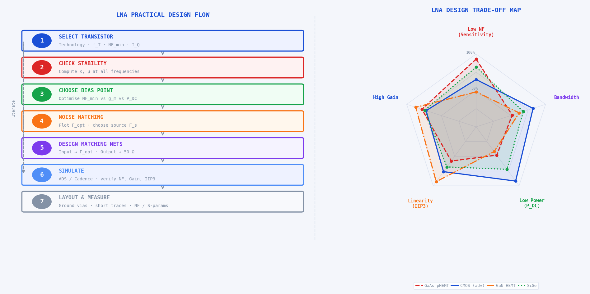
The choice of semiconductor technology is the most fundamental decision in LNA design and constrains every subsequent design parameter. The diagram above illustrates the trade-off profile of each major technology across the five key LNA performance dimensions.
GaAs pHEMT remains the gold standard for low-NF applications (satellite, GNSS, radio astronomy) where cost is secondary to performance. The 2DEG (two-dimensional electron gas) channel provides very high electron mobility and extremely low channel thermal noise.
Advanced CMOS (28 nm and below) has closed the NF gap significantly in the last decade, reaching NF_min below 1 dB at 5 GHz in 28 nm bulk CMOS. Its dominant advantage is integration density — the entire receiver (LNA, mixer, VCO, baseband, ADC) integrates on a single die, dramatically reducing cost at volume. The primary limitation is lower breakdown voltage (1.8 V max for 28 nm) which limits headroom and output power.
GaN HEMT is not typically used for ultra-low-NF front ends. Its strengths are high breakdown voltage (100+ V), extremely high power density (10+ W/mm), and good linearity (IIP3 up to +40 dBm). It dominates radar and electronic warfare LNA/PA designs where large input signals must be handled without compression.
SiGe BiCMOS combines the high f_T and low NF of SiGe HBTs (heterojunction bipolar transistors) with the integration density of CMOS digital circuits. It is the technology of choice for 5G base-station front-ends and automotive radar (77 GHz), where sub-1 dB NF, moderate power, and silicon-scale integration are all required simultaneously.
Bandwidth Considerations
Narrowband vs Broadband LNAs
The choice of narrowband versus broadband architecture is driven by the application's frequency plan. A narrowband LNA is designed to operate over a fractional bandwidth of typically less than 10% (e.g., 2.40–2.48 GHz for 2.4 GHz Wi-Fi). A broadband LNA must maintain flat gain and low NF over multiple octaves (e.g., 0.5–6 GHz for a software-defined radio front end).
Narrowband designs achieve the best NF and highest gain — the resonant input matching network at Γ_opt provides a noise boost at the design frequency that simply is not available to broadband designs. Broadband designs sacrifice NF (typically 1–3 dB worse than narrowband at the same frequency) in exchange for flexibility and coverage.
Broadband Techniques
- Resistive feedback (shunt-feedback). As covered in Part 2, a feedback resistor from drain to gate flattens the gain response and provides a wideband 50 Ω input match. The NF floor is set by the feedback resistor's thermal noise — typically 2–4 dB across a multi-octave band. Variants include the common-gate common-source combined topology (CGCS) which allows simultaneous noise and power matching over a wider band.
- Distributed (travelling-wave) amplification. The transistor input capacitances are absorbed into artificial transmission line sections, creating a structure with inherently flat gain from near-DC to millimetre-wave. The NF is moderate (3–6 dB) because each transistor's noise is not coherently combined, but the bandwidth can exceed a decade. Used in test equipment, electronic warfare, and ultra-wideband (UWB) radar.
- Noise-cancelling topology. A feedforward path cancels the noise of the main amplifier transistor while the signal passes through constructively. In principle this allows both wideband operation and NF approaching 0 dB. Practical implementations achieve NF of 1–2 dB over multi-octave bandwidth. Covered in detail in Section 20.
- Transformer-coupled matching. A wideband transformer (Balun or Marchand balun) converts the complex transistor input impedance to 50 Ω over a wide frequency range. Used in differential LNA designs at RF and microwave frequencies.
- Frequency-selective gain equalisation. For multi-band applications (e.g., a 5G FR1 + FR2 LNA), switchable matching networks (PIN diodes, RF MEMS, or varactors) reconfigure the input match for each band. NF is near-optimal in each band, but the switch adds loss and the control logic adds complexity.
Practical Design Flow
The seven-step flow illustrated in the diagram above is the systematic process used in industry from initial specification to taped-out silicon or manufactured PCB. Each step feeds back into the previous ones — the process is iterative, not linear.
Step 1 — Select the Transistor
The transistor sets the fundamental limits: NF_min, available gain, IIP3, and maximum operating frequency. Key selection criteria: f_T ≥ 5× f_design (for 10 dB gain margin at the design frequency); NF_min ≤ (target NF − 0.5 dB) to allow for matching network imperfections; foundry PDK availability for simulation; and packaging that matches the PCB or MMIC process.
Step 2 — Check Stability at All Frequencies
Before any matching network is designed, extract the bare transistor S-parameters at the chosen bias point and compute μ and K from DC to 3× f_design. If the device is potentially unstable (μ < 1 at any frequency), apply a stabilisation technique (Section 10 of Part 2) before proceeding. It is far easier to stabilise the transistor before matching networks constrain the impedance environment.
Step 3 — Choose the Bias Point
Sweep I_DS from 10% to 80% of I_DS,max and plot NF_min vs I_DS at the design frequency. Identify the bias current that achieves the target NF_min with acceptable P_DC. For narrowband designs, also check that the gain and IIP3 at this bias point meet the Friis budget requirements established in the system design phase.
Step 4 — Perform Noise Matching
Extract the four noise parameters (NF_min, R_n, Γ_opt, G_assoc) at the chosen bias point from the transistor model or measurement. Plot noise circles for NF = NF_min + 0.5 dB and NF_min + 1 dB on the Smith chart. Overlay available gain circles. Choose a source reflection coefficient Γ_s inside both the acceptable noise circle and a gain circle that satisfies the link budget. This Γ_s is the target for the input matching network.
Step 5 — Design the Matching Networks
Design the input matching network to transform the 50 Ω source to the chosen Γ_s. Design the output matching network independently to conjugate-match the transistor output to 50 Ω (maximising power transfer to the next stage). Use Smith chart rotation for distributed (transmission line) networks, or LC ladder synthesis for lumped networks. Include component Q factors in the design — real inductors and capacitors have finite Q that degrades NF and return loss from the ideal values.
Step 6 — Simulate
Full-wave or circuit simulation is mandatory before fabrication. Key simulations: S-parameter sweep (verify gain, NF, S11, S22, stability); noise figure simulation (verify NF vs frequency, NF vs bias); two-tone IIP3 sweep (verify linearity budget); and temperature sweep (−40 to +85°C) to check for bias drift and stability at temperature extremes. If the design uses PCB transmission lines, EM simulate the matching network layout to capture radiation resistance, coupling, and parasitic capacitance.
Step 7 — Layout Considerations and Measurement
PCB layout for RF circuits follows rules that are fundamentally different from digital or analogue design:
- Ground vias directly under and around the LNA. Every millimetre of ground inductance degrades gain, NF, and stability. Use via arrays — not a single via — for the transistor source/emitter ground.
- Shortest possible RF input trace. Every parasitic capacitance and inductance on the input trace shifts the matching network away from Γ_s. Use CPW (coplanar waveguide) for better-controlled impedance on thin substrates.
- Separation of RF and DC bias routing. Route DC bias traces perpendicular to the RF signal path. Use RF chokes (high-impedance inductors) or λ/4 high-impedance stubs at the RF frequency to present open circuits to RF at supply pins.
- Component placement for thermal management. The LNA transistor and bias resistors generate heat. For high-power GaN or PA-adjacent designs, thermal vias and copper planes conduct heat to the PCB backside.
Simulation Tools
Keysight ADS (Advanced Design System)
ADS is the industry-standard circuit and system simulator for RF and microwave design. For LNA work it provides: harmonic balance simulation for IIP3 and P1dB; noise simulation using the four-noise-parameter model; S-parameter simulation for gain and stability; momentum EM simulation for passive structures (microstrip lines, via transitions, matching stubs); and co-simulation coupling circuit schematics to EM-simulated layout. ADS datasheets export S2P files directly compatible with VNA measurement software. Most MMIC foundry PDKs are delivered as ADS design kits with process-accurate transistor models.
Ansys HFSS
HFSS is a full-wave 3D electromagnetic field simulator based on the finite-element method (FEM). It is used for LNA layout effects that circuit simulators cannot capture: connector and via transitions at mmWave frequencies; package coupling between the LNA chip and its PCB environment; radiation resistance of PCB traces acting as unintended antennas; and cavity resonances in metallic LNA housings. HFSS exports S-parameters as Touchstone files that feed back into ADS or Cadence for co-simulation. At frequencies above 10 GHz, HFSS is often essential for design closure — layout effects at 28 GHz can shift resonances by hundreds of MHz from the schematic prediction.
Cadence Virtuoso / Spectre RF
For integrated circuit LNA design in CMOS or SiGe BiCMOS, Cadence Virtuoso is the dominant environment. The foundry PDK provides calibrated transistor SPICE models (BSIM4 for CMOS, VBIC for SiGe HBT) that include layout-dependent effects (LDE): threshold voltage shifts from well proximity effect, gate resistance from finger layout, and substrate coupling. Spectre RF (part of Virtuoso) supports periodic steady-state (PSS) analysis for IIP3, phase noise, and conversion gain. Virtuoso's electromagnetic simulation (EMX or Virtuoso EM) handles on-chip inductors, transformers, and coupling between metal layers at the transistor level — effects that are critical for on-chip matching network design above 20 GHz.
Simulation accuracy is only as good as the model accuracy. Transistor models are calibrated at specific bias points and frequencies — extrapolating outside this range degrades accuracy. At mmWave frequencies (above 30 GHz), parasitic extraction from layout becomes as important as the transistor model itself. Always validate the first silicon or PCB prototype against simulation, identify discrepancies, and update models before re-spinning. A good simulation-to-hardware correlation is ±0.3 dB on NF and ±0.5 dB on gain at the design frequency.
Measurement and Characterisation
Noise Figure Measurement
Noise figure is measured using one of two approaches. The Y-factor method with a calibrated noise source is the most common and is automated in modern noise figure analysers (Keysight N8975B, Rohde & Schwarz FSVR):
- Connect the calibrated noise source (known ENR — Excess Noise Ratio, typically 5–15 dB) to the LNA input.
- Measure the output power with the noise source ON (T_hot ≈ 10,000 K) and OFF (T_cold = T₀ = 290 K).
- The Y-factor Y = P_hot/P_cold, from which F is calculated as described in Part 1.
- The analyser itself has a noise figure NF_analyser that must be subtracted from the raw measurement using the Friis formula. This subtraction (called "DUT calibration" or "second-stage correction") is performed automatically.
Measurement uncertainty in NF is dominated by: ENR calibration uncertainty of the noise source (±0.1–0.3 dB), mismatch between the noise source and the LNA input (corrected with impedance correction factors), and the analyser's own noise figure after correction. Well-calibrated setups achieve ±0.1 dB NF measurement uncertainty at 1–10 GHz, degrading to ±0.3–0.5 dB above 26 GHz.
S-Parameter Measurement
S-parameters are measured with a Vector Network Analyser (VNA). The measurement procedure for an LNA:
- Calibration. Perform a full 2-port SOLT (Short-Open-Load-Thru) or multiline TRL calibration to move the reference planes to the LNA's input and output connectors. At mmWave frequencies, on-wafer probing with LRRM or SOLR calibration is used.
- Power level setting. The VNA source power must be set well below the LNA's P1dB (typically −30 to −20 dBm at the LNA input) to ensure linear operation. If the VNA source power is too high, the measured S21 will be lower than the small-signal gain.
- Receiver attenuation. The VNA's receiver must be protected from the LNA output power. Use a fixed attenuator (10–20 dB) between the LNA output and the VNA port 2 receiver, then de-embed the attenuator from the S-parameter results.
- DC bias application. Supply the LNA's DC bias through bias tees on both VNA ports. Verify the DC operating point (I_DS, V_DS) with a multimeter before taking RF measurements.
Gain and Linearity Testing
Large-signal gain and P1dB are measured with a signal generator and a spectrum analyser or power meter. Sweep the input power from −40 dBm to above the expected P1dB in 1 dB steps. Plot output power vs input power. The 1 dB compression point is where the measured output power falls 1 dB below the extrapolated linear fit.
IIP3 is measured with a two-tone test. Two signal generators at f1 and f2 (typically 1 MHz apart, both in-band) drive the LNA through a combiner. A spectrum analyser measures the fundamental tones (at f1 and f2) and the IM3 products (at 2f1−f2 and 2f2−f1). IIP3 is calculated from the measured power levels using the formula in Part 2. Tone spacing should be narrow enough to keep both tones within the LNA's passband, but wide enough that IM3 products are resolvable from the fundamental on the spectrum analyser.
Advanced Topics
Cryogenic LNAs
At temperatures below 20 K (achievable with liquid helium or pulse-tube cryocoolers), electron mobility in GaAs and InP HEMTs increases dramatically and the channel thermal noise power kTB approaches zero. Cryogenic LNAs achieve noise temperatures below 5 K at 1–10 GHz — equivalent to NF below 0.07 dB. They are used in:
- Radio astronomy (Atacama Large Millimeter Array, Very Large Array receiver chains)
- Quantum computing readout chains (superconducting qubit control and measurement at 4 K)
- Deep-space network receivers (NASA DSN 70-metre dishes for interplanetary communication)
The design principles are identical to room-temperature LNAs, but biasing must account for the temperature dependence of V_th (which shifts by 50–200 mV between 300 K and 15 K), and all passive components must maintain their specifications at cryogenic temperatures. Cryogenic coaxial cables and connectors introduce unique considerations — differential thermal contraction and moisture absorption that degrades performance on thermal cycling.
mmWave LNAs (24–300 GHz)
LNA design above 24 GHz (5G FR2, automotive radar at 77 GHz, imaging at 94 GHz, D-band backhaul at 140 GHz) differs fundamentally from sub-6 GHz design in several respects:
- Transistor parasitics dominate. At 28 GHz, a 0.1 pF parasitic capacitance presents only 57 Ω — comparable to the matching impedance. Layout extraction becomes inseparable from the schematic design. Full EM-circuit co-simulation is mandatory.
- Transmission lines replace lumped elements. Inductors with self-resonance above 50 GHz do not exist in standard processes. All matching is done with microstrip or CPW stubs, transmission line transformers, or Lange couplers.
- Gain per stage decreases with frequency. At 77 GHz, a single cascode stage provides 8–12 dB. Multiple cascaded stages are required for total system gain — raising the importance of inter-stage matching and stability at each interface.
- NF is inherently higher. At 77 GHz, state-of-the-art CMOS LNA NF is 5–7 dB; GaAs and InP can reach 2–3 dB. The fundamental reason is increased transistor noise current at high frequencies (gate current noise ∝ ω²C²_gs) and increased resistive losses in passive components.
Differential LNAs
Differential LNAs use two matched transistors driven by balanced (differential) signals — 180° out of phase. Common-mode noise (supply noise, substrate coupling, interferers coupling equally into both signal paths) is rejected. Differential architectures are dominant in integrated receivers where the LNA output drives a double-balanced mixer. Key advantages:
- Common-mode rejection ratio (CMRR) typically > 40 dB — supply noise is suppressed equally
- Second-order distortion cancels — IM2 products are common-mode and rejected
- Improved IIP3 at the same bias current compared to single-ended (the differential pair linearises the transconductance)
The main cost is doubled power consumption and the need for a balun (balanced-to-unbalanced converter) at the antenna interface, which adds insertion loss at the most noise-sensitive point in the chain.
Noise Cancellation Techniques
Noise cancellation LNAs exploit a key property of the common-gate topology: the noise of the input transistor M1 appears with the same phase at the input node, but with opposite phase at the output node (since the output is inverted by the gain of the stage). A feedforward path from the input to a second summation amplifier adds the input-referred noise constructively — and the two contributions cancel at the final output. The signal, meanwhile, adds constructively in both paths.
The noise cancellation condition requires the gain of the feedforward path to exactly match the magnitude of the main path noise — a condition sensitive to component matching. In practice, noise cancellation provides 10–20 dB of input transistor noise rejection, reducing the total NF by 1–3 dB while maintaining wideband operation. Published results show 1.5–2.5 dB NF across 0.5–6 GHz bandwidth in 65 nm CMOS — competitive with narrowband GaAs designs at a fraction of the cost.
Machine Learning in RF Design
Machine learning is beginning to enter RF and microwave design workflows, though it remains an emerging rather than established practice. Current applications include:
- Surrogate modelling. Neural networks trained on EM simulation results (S-parameters vs geometry) enable near-instantaneous evaluation of layout variants that would take hours in HFSS. Gradient descent through the surrogate model then optimises matching network geometry directly.
- Automated bias optimisation. Reinforcement learning agents can sweep the transistor bias point and simultaneously optimise NF, gain, and IIP3 within a circuit simulator, finding Pareto-optimal bias points faster than human-guided sweeps.
- Yield prediction and process variation management. Monte Carlo simulation of process corners produces training data for a classifier that predicts whether a given design will meet spec across the full process distribution — enabling early-stage yield optimisation without full Monte Carlo runs.
- Topology selection. Graph neural networks trained on databases of published LNA circuits can recommend starting topologies given a set of specifications (frequency, NF target, technology, power budget) — shortcutting the literature review phase of design.
The key limitation today is training data volume — RF design databases are orders of magnitude smaller than the image or language datasets that drive mainstream ML. This constraint is easing as foundries and EDA vendors build proprietary simulation datasets, and as physics-informed neural networks (PINNs) reduce the data requirement by encoding Maxwell's equations into the model architecture.
Design Trade-offs Summary
Every LNA design navigates the five-way tension illustrated in the radar chart above. No single topology or technology excels in all five dimensions simultaneously. Understanding the trade-offs is the hallmark of an experienced RF engineer. The table below consolidates the key relationships across the entire three-part series:
✓✓ = significant improvement · ✓ = moderate improvement · – = negligible effect · ✗ = moderate penalty · ✗✗ = significant penalty
No LNA ever achieves best-in-class performance in all five dimensions. A satellite LNA (GaAs, NF = 0.4 dB) draws 80 mA and costs $15/unit. An IoT LNA (CMOS, NF = 2.2 dB) draws 1.2 mA and costs $0.08/unit. A radar LNA (GaN, IIP3 = +30 dBm) draws 200 mA and handles 1 W of input power without damage. Each is the right design for its application. The job of the RF engineer is not to design the theoretically best LNA — it is to design the best LNA for a specific set of constraints. Defining those constraints precisely, from system-level specifications down to transistor bias point, is exactly what this three-part series has equipped you to do.
Questions & Worked Examples
Work through each problem fully before reading the solution.
Current Mirror Bias — Choosing W/L for Target I_DS
Problem: A 28 nm CMOS LNA requires I_DS = 8 mA at V_GS = 0.65 V. The reference transistor M_ref has W_ref/L = 10 μm/28 nm and carries I_ref = 200 μA from a bandgap reference. Find: (a) the required W1/L of the LNA transistor M1, (b) the mirroring ratio W1/W_ref, (c) if process variation shifts I_ref by +10%, what is the new I_DS?
The current mirror tracks I_ref linearly — a 10% change in I_ref produces an equal 10% change in I_DS. This is far better than a resistive divider bias, where a 10% VDD variation causes a non-linear V_GS shift that can move the transistor out of saturation or into the NF_min sweet spot. The mirror ratio of 40:1 requires careful layout — both transistors must share the same well, orientation, and be interdigitated (common-centroid layout) to minimise threshold voltage mismatch from process gradients. Threshold mismatch ΔV_th between M_ref and M1 causes a systematic current error: ΔI_DS ≈ 40 × g_m,ref × ΔV_th.
Technology Selection — GaAs vs CMOS for a 5G Sub-6 GHz LNA
Problem: You are designing an LNA for a 5G NR n78 band (3.3–3.8 GHz) base-station receiver. Specifications: NF ≤ 1.2 dB, Gain ≥ 18 dB, IIP3 ≥ 0 dBm, P_DC ≤ 50 mW, volume price target < $0.50/unit at 100k units. Two candidates are shortlisted:
Option A: GaAs pHEMT MMIC — NF = 0.7 dB, Gain = 22 dB, IIP3 = +5 dBm, P_DC = 45 mW, price = $3.20/unit
Option B: 28 nm CMOS integrated — NF = 1.1 dB, Gain = 19 dB, IIP3 = +2 dBm, P_DC = 18 mW, price = $0.18/unit
Which option meets all specifications? Which is the better engineering choice for this application, and why?
GaAs Option A fails the price specification outright — $3.20 vs a $0.50 target, and the volume price for GaAs MMICs does not decrease significantly at 100k units (it would need millions). CMOS Option B meets every specification including price, draws 60% less power (reducing cooling requirements in densely packed base-station radio units), and integrates with the digital beamforming ASIC on the same die in a full SoC solution. The 0.4 dB NF advantage of GaAs is real but irrelevant here — the system specification is 1.2 dB and the CMOS achieves 1.1 dB with 0.1 dB of margin. GaAs would be the correct choice only if NF ≤ 0.8 dB were required (e.g., for a tower-mounted LNA in a rural macro cell where link budget is tight and cost is secondary).
Y-Factor NF Measurement — Correcting for Second Stage
Problem: A noise figure analyser (NFA) with NF_NFA = 6.5 dB measures an LNA. The noise source has ENR = 15.0 dB. With the LNA connected, the NFA reads NF_meas = 7.8 dB (this includes the NFA's own noise). Calculate the true LNA noise figure, corrected for the NFA's second-stage contribution.
With 20 dB LNA gain, the NFA second-stage correction is only 0.03 dB — negligible. This confirms why high-gain LNAs are easy to measure accurately with even a mediocre NFA. If the LNA gain were only 6 dB (G = 4 linear), the second-stage correction would be (4.467−1)/4 = 0.867, and the corrected NF would be 6.026 − 0.867 = 5.159 → 7.13 dB — a 0.67 dB correction. This is why measurement accuracy matters most for low-gain, low-NF LNA stages, and why the NFA's own NF should be specified and verified before any critical measurement.
Trade-off Analysis — Narrowband vs Broadband for SDR Front End
Problem: A software-defined radio (SDR) front end must cover 0.5–6 GHz. Two architectures are proposed:
Architecture N: Four switchable narrowband inductively-degenerated LNAs, each covering a 1.5 GHz sub-band. Each achieves NF = 1.0 dB and IIP3 = −2 dBm in its band. Switch insertion loss = 1.0 dB. Total P_DC = 80 mW (all four always powered).
Architecture B: Single broadband noise-cancellation LNA covering 0.5–6 GHz. NF = 2.2 dB flat, IIP3 = +3 dBm, P_DC = 45 mW.
For a 10 MHz channel at 3.5 GHz requiring SNR_min = 20 dB, calculate the receiver sensitivity for each architecture and state which is better and why.
The narrowband architecture's 1.0 dB NF advantage is almost entirely cancelled by the 1.0 dB switch insertion loss — a textbook illustration of the pre-LNA loss rule. The sensitivity difference is only 0.2 dB — essentially equivalent in practice. Architecture B wins on total power (45 vs 80 mW), component count, and board space. Architecture N wins on IIP3 (−2 vs +3 dBm) and on flexibility to individually optimise each band. For an SDR where a strong adjacent-channel interferer is the primary concern, Architecture N's IIP3 advantage (+5 dBm better) justifies its complexity. For a general-purpose SDR where linearity and sensitivity are balanced, Architecture B is the better system-level choice. This is the kind of trade-off that must be resolved at system level, not at LNA level alone.