LNA Design — Noise Parameters, Stability, Topologies and Linearity

Fig 1 — Six LNA circuit topologies with schematic thumbnails and key characteristics

Six LNA topology diagrams: Common Source, Common Gate, Inductive Degeneration, Cascode, Resistive Feedback, and Current Reuse — each with schematic and key characteristics

Noise Parameters

In Part 1 we defined noise figure as a single number — the SNR degradation through a device. But NF is not a fixed property of an amplifier. It depends on the source impedance presented to the transistor's input. The complete description of a transistor's noise performance requires four quantities known collectively as the noise parameters.

NF_min — Minimum Achievable Noise Figure

NF_min (also written F_min or NF_opt) is the lowest noise figure the transistor can achieve — the floor set by the device physics, independent of circuit design. It is reached only when the source reflection coefficient equals the optimum noise reflection Γ_opt exactly. NF_min improves (decreases) with:

Lower operating frequency (transistors are less noisy at lower f)
Higher transistor f_T (transition frequency) — faster devices have lower NF_min
Reduced channel length in CMOS (shorter = faster = lower NF_min)
Optimum DC bias current (NF_min has a minimum vs I_DS)

NF_min is a datasheet-specified parameter, measured at a specific frequency, bias, and temperature. It is always the starting benchmark — no matching network can reduce the NF below NF_min.

R_n — Noise Resistance

The noise resistance R_n (in ohms) governs the sensitivity of NF to source impedance mismatch from Γ_opt. It is not a physical resistor — it is a normalisation constant that appears in the NF equation. A high R_n means NF degrades rapidly as the source moves away from Γ_opt; a low R_n means the design is tolerant of source impedance variation:

Noise figure as a function of source reflection coefficient

NF = {NF}_{\min} + \frac{4 R_{n} {| Γ_{s} - Γ_{opt} |}^{2}}{Z_{0} (1 - {| Γ_{s} |}^{2}) {| 1 + Γ_{opt} |}^{2}}

R_n appears in the numerator — larger R_n → steeper NF penalty for any given |Γ_s − Γ_opt|. Typical values: R_n = 5–50 Ω. A transistor with R_n/Z₀ ≪ 1 is more forgiving of matching errors.

Γ_opt — Optimum Source Reflection Coefficient

Γ_opt is the complex source reflection coefficient that minimises NF to NF_min. It is a point on the Smith chart — and in general it is not at the centre (50 Ω), nor does it equal S11*. Γ_opt is typically in the inductive quadrant (upper half of the Smith chart) for MOSFET transistors at RF frequencies, because the gate-source capacitance C_gs must be resonated for optimum noise performance.

The input matching network's role in a noise-optimised LNA is to transform the 50 Ω source impedance Z₀ to the impedance corresponding to Γ_opt — bringing the source to the optimal noise point on the Smith chart.

Noise Circles — Constant NF Contours

Loci of constant noise figure in the Γ_s plane are circles on the Smith chart, called noise circles. Every noise circle corresponds to a specific NF value and is centred on the line connecting Γ_opt to the centre of the Smith chart. The innermost noise circle (radius → 0) corresponds to NF = NF_min and degenerates to the single point Γ_opt.

The centre and radius of the noise circle for NF = NF_i are:

Noise circle centre C_Ni and radius r_Ni

C_{N i} = \frac{Γ_{opt}}{N_{i} + 1} r_{N i} = \frac{\sqrt{N_{i}^{2} + N_{i} (1 - {| Γ_{opt} |}^{2})}}{N_{i} + 1}

N_i = (F_i − F_min)|1 + Γ_opt|² / (4R_n/Z₀), where F_i = 10^(NF_i/10). As NF_i increases from NF_min, N_i increases from 0 and the circle expands outward from Γ_opt.

Smith Chart for LNA Design

Noise Circles and Gain Circles

The complete LNA design problem is solved graphically by plotting two families of circles on the Smith chart:

Noise circles (red, centred near Γ_opt in upper Smith chart) — each circle is a contour of constant NF. The innermost circle is NF_min at Γ_opt.
Available gain circles (blue, centred near S11*) — each circle is a contour of constant available gain G_A. The maximum gain circle degenerates to the point Γ_s = S11* (conjugate match).

Fig 2 — Smith chart showing noise circles, gain circles, and the design trade-off region

The design workflow proceeds as follows:

Plot noise circles for acceptable NF contours (e.g., NF_min, NF_min+0.5 dB, NF_min+1 dB).
Plot available gain circles for desired G_A values.
Identify the design region — Γ_s values that simultaneously satisfy NF ≤ target and G_A ≥ target.
Choose a specific Γ_s in that region, then design the input matching network to transform 50 Ω to that Γ_s.
Design the output matching network independently to present Γ_L = Γ_out* for maximum power transfer to the next stage.

📌 Simultaneous Noise and Power Match (SNPM)

When Γ_opt ≈ S11*, the noise and gain circles overlap almost completely and a single matching network achieves both objectives simultaneously. Inductively degenerated LNAs are specifically engineered to realise this condition at the design frequency by choosing L_s to move the transistor's effective Γ_opt toward S11*.

Stability Considerations

Conditional vs Unconditional Stability

An amplifier is unconditionally stable if it cannot oscillate for any combination of passive source and load impedances. It is conditionally stable (potentially unstable) if there exist source or load impedances — even passive ones — that cause the amplifier to oscillate. Oscillation occurs when the real part of the input or output impedance becomes negative, which happens when feedback from output to input is large enough relative to the gain.

At RF frequencies, every transistor has a non-zero reverse transmission (S12 ≠ 0) — energy leaks from the output back to the input through the gate-drain capacitance C_gd. If this feedback is not managed, the LNA can oscillate, producing spurious tones, rendering the receiver useless, and potentially damaging other components.

Rollett Stability Factor K

The most widely used stability criterion is the Rollett factor K combined with the condition |Δ| < 1:

Rollett stability factor K

K = \frac{1 - {| S_{11} |}^{2} - {| S_{22} |}^{2} + {| Δ |}^{2}}{2 | S_{12} S_{21} |}

Δ = S11·S22 − S12·S21 is the determinant of the S-matrix. Unconditional stability requires K > 1 AND |Δ| < 1, both simultaneously at every frequency. Either condition alone is insufficient.

An alternative single-parameter criterion that is both necessary and sufficient is the μ-factor:

μ-factor stability criterion (necessary and sufficient alone)

μ = \frac{1 - {| S_{11} |}^{2}}{| S_{22} - Δ^{*} S_{11} | + | S_{12} S_{21} |} > 1

μ > 1 is sufficient (and necessary) for unconditional stability. Unlike the K-|Δ| pair, a single μ value determines stability. A larger μ means a larger stability margin — more robust against component variations and parasitic impedances.

Stability Circles

For a conditionally stable device (K < 1), stability circles on the Smith chart show which source and load impedance regions cause instability. The input stability circle is the boundary in the Γ_s plane beyond which the output reflection coefficient |Γ_out| ≥ 1. The output stability circle is the boundary in the Γ_L plane beyond which |Γ_in| ≥ 1.

The LNA designer must ensure the chosen Γ_s (from the noise/gain design) lies entirely within the stable region of the source stability circle — and check this at all frequencies, not just the design frequency.

Stabilisation Techniques

When a transistor is potentially unstable, the following techniques restore stability, each at a cost:

Technique	How it works	Cost
Series gate/base resistor	Small R (10–50 Ω) in series with gate reduces gain at low freq where K < 1	Adds thermal noise → NF penalty
Parallel RC at input	R in series with C shunted to ground — acts at low freq only, transparent at design freq	Minimal NF impact if C chosen correctly
Resistive drain termination	Shunt R at output port reduces output reflection and feedback path gain	Reduced gain; higher output noise
Cascode topology	Common-gate M2 shields C_gd of M1, dramatically reducing S12	Slightly higher voltage headroom required
Source degeneration inductor	L_s modifies the transistor's effective S11, moving the stability boundary	Slightly reduced gain; may affect NF

📌 Check Stability at Every Frequency

Transistors are most dangerous at frequencies away from the design point — particularly below 1 GHz where gain is highest. An LNA stable at 5.8 GHz may oscillate at 500 MHz if the matching networks present a reactive load at that frequency. Always compute K and μ from near-DC to several times f_design before finalising a design.

LNA Topologies

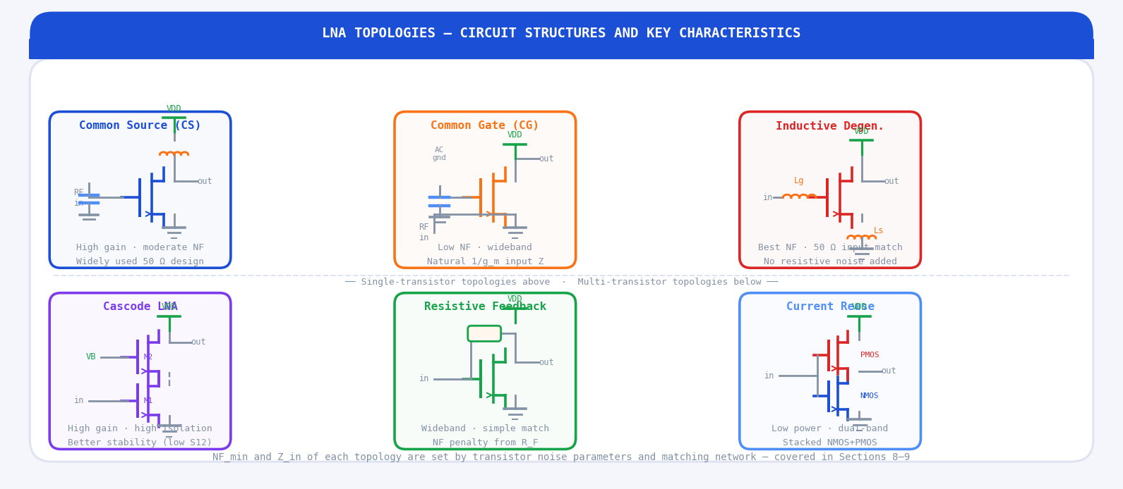
Common Source (CS)

The common-source configuration is the RF equivalent of the common-emitter: the gate is the input, the drain is the output, and the source is the AC ground (bypassed to ground through a decoupling capacitor). It provides the highest voltage gain of any single-transistor configuration and is the workhorse topology for moderate-bandwidth LNA designs.

The basic CS LNA, however, presents a purely capacitive input impedance (≈ 1/jωC_gs), so a matching network is mandatory for 50 Ω input. The input matching network's impedance transformation ratio increases the effective noise figure above NF_min unless carefully designed. Without any feedback mechanism, simultaneous noise and power match requires an input matching network that transforms 50 Ω to Γ_opt — but this exact match is only possible over a narrow bandwidth.

Common Gate (CG)

In the common-gate configuration the gate is AC-grounded, the input is at the source, and the output is at the drain. The small-signal input impedance looking into the source is approximately 1/g_m — and by choosing the transistor bias to set g_m = 1/50 = 20 mS, the input is inherently matched to 50 Ω without any external matching network. This makes the CG topology attractive for wideband designs.

The noise figure of an ideal CG stage is limited by:

Minimum NF of common-gate LNA

{NF}_{CG,min} \approx 10 {log}_{10} (1 + γ) dB

γ is the transistor's channel noise factor (≈ 2/3 for long-channel MOSFET, but can reach 2–4 in short-channel devices). Minimum CG NF ≈ 10 log(1 + 2/3) = 2.2 dB — worse than a well-designed CS or inductive degeneration LNA but simpler and inherently wideband.

Common Drain (CD) / Source Follower

The common-drain (source follower) has unity voltage gain and is not used as an LNA gain stage. It is valuable as a buffer: it presents high input impedance to the LNA and low output impedance (≈ 1/g_m) to drive a subsequent low-impedance load such as a transmission line or mixer. In some multi-stage LNA designs a CD stage follows the gain stage to drive the mixer directly.

Inductively Degenerated LNA

The inductively degenerated (or source-degenerated) LNA is the dominant topology for narrowband, low-NF applications. A source degeneration inductor L_s is inserted between the transistor source and ground, and a gate inductor L_g tunes out the combined reactance. The result is a real input impedance of approximately 50 Ω achieved without any resistor — so the 50 Ω match adds no thermal noise.

The resonant input impedance was derived in Part 1:

Input impedance of inductively degenerated LNA at resonance

Z_{in} = \frac{g_{m} L_{s}}{C_{gs}} + j ω (L_{g} + L_{s}) - \frac{j}{ω C_{gs}}

Setting the imaginary part = 0 (resonance) gives ω₀² = 1/[(L_g + L_s)C_gs]. At resonance, Z_in = g_m·L_s/C_gs = ω_T·L_s, where ω_T = g_m/C_gs is the transistor unity-gain frequency. Set L_s = Z₀/ω_T to achieve Z_in = 50 Ω.

The key advantage: L_s shifts the transistor's effective Γ_opt toward S11*, enabling simultaneous noise and power match over a narrow frequency range. The resulting NF is very close to NF_min, achievable simultaneously with good input return loss — no compromise required.

Cascode LNA

The cascode places a common-gate transistor M2 above a common-source M1, with M1's drain connected to M2's source. The common-gate M2 acts as a buffer — it presents low impedance to M1's drain (suppressing the Miller effect on C_gd), and isolates the output from the input by reducing S12 by a factor of approximately g_m2·r_o1. Key advantages over single-transistor CS:

Higher gain (the gain is approximately g_m1·R_L, same as CS, but bandwidth is higher due to reduced Miller capacitance)
Much lower S12 — dramatically improved reverse isolation, making stability easier to achieve and maintain
Higher output impedance — simplifies output matching to 50 Ω

The noise figure of a cascode is approximately the same as the CS stage alone if the transconductance of M2 is sufficiently large, because M2 is a common-gate stage and its noise contribution is suppressed by M1's gain preceding it.

Resistive Feedback LNA

A resistor R_F connected from drain to gate provides wideband negative feedback that simultaneously broadens the frequency response and improves the input match. The input impedance is approximately:

Input impedance of resistive feedback LNA

Z_{in} \approx \frac{R_{F} + R_{L}}{1 + g_{m} R_{L}}

Choosing R_F and R_L so that Z_in = 50 Ω gives a wideband match. The trade-off: R_F contributes thermal noise (temperature T, resistance R_F) directly at the input — NF is higher than inductive degeneration, but bandwidth is far greater. Typical NF: 2–4 dB over multi-octave bandwidth.

Current Reuse LNA

The current reuse topology stacks an NMOS transistor (input) and a PMOS transistor (output) in series between VDD and GND. Both transistors are biased from the same DC current path — the NMOS drain current is reused as the PMOS source current. Both transistors' RF inputs are driven by the same signal (their gates are AC-coupled together), effectively doubling the transconductance for the same DC power consumption:

Effective transconductance of current reuse stage

G_{m} = g_{m 1} + g_{m 2}

For matched NMOS/PMOS pairs with equal transconductance: G_m = 2g_m at the same I_DD as a single-transistor stage. Gain doubles (6 dB) for no additional power — highly attractive for IoT and battery-powered designs where P_DC ≤ a few milliwatts.

The NF of a current reuse LNA can approach that of an inductive degeneration LNA when combined with appropriate source degeneration on both transistors. The main design challenges are the tighter headroom (VDD must accommodate both transistors), PMOS transistors' inferior noise performance vs NMOS at RF, and the need for careful bias design to keep both transistors in saturation.

Impedance Matching Networks

Lumped vs Distributed Matching

Impedance matching networks transform the source or load impedance to the value required at the transistor's port. Two implementation families exist:

Lumped element matching uses discrete inductors and capacitors (or their on-chip equivalents). Compact, narrowband, frequency-agile (values can be tuned). Preferred below ~5 GHz where component sizes are small relative to λ.
Distributed matching uses transmission line sections — microstrip stubs, quarter-wave transformers, open or shorted lines. Naturally suited above 5 GHz where lumped component parasitics dominate, and for PCB-integrated LNA designs.

L-Section Matching Network

The L-network is the simplest two-element matching circuit. It transforms a source impedance R_s to a load impedance R_L using one series and one shunt reactive element. The required Q and element values are:

L-network matching Q factor

Q = \sqrt{\frac{R_{high}}{R_{low}} - 1}

R_high is the larger of R_s and R_L. The shunt element goes in parallel with the larger resistance; the series element goes in series with the smaller. For R_s = 50 Ω to R_L = 200 Ω: Q = √(200/50 − 1) = √3 ≈ 1.73. The −3 dB bandwidth of the match is f₀/Q.

For a high-Q match (large impedance transformation ratio), the L-network has a narrow bandwidth. For wideband operation, a ladder network (multiple L-sections) or a distributed network is needed.

Transmission Line Stub Matching

A single transmission line stub (open or shorted) in parallel with the signal path can cancel the reactive part of the load impedance, leaving a real impedance to match with a series line section. The stub length is chosen to present the required susceptance at the design frequency:

Susceptance of a shorted stub of electrical length θ = βl

B = \frac{1}{Z_{0} tan (θ)}

For an open stub: B = −1/(Z₀ tan θ). Choosing θ so that B cancels the load susceptance leaves a real impedance. A second line section then transforms this real impedance to 50 Ω. The complete procedure is performed graphically using the Smith chart — rotate along constant-|Γ| arcs.

Quarter-Wave Transformer

A transmission line section of exactly λ/4 electrical length (θ = 90°) transforms a real load impedance R_L to a real input impedance R_in through:

Quarter-wave transformer

Z_{0} = \sqrt{R_{in} \cdot R_{L}}

Choose the transformer's characteristic impedance as the geometric mean of source and load. Works only for real (resistive) impedances. For complex loads, first resonate out the reactance with a series stub, then apply the quarter-wave transformer to the resulting real impedance.

Quarter-wave transformers are used extensively in balanced LNA designs (between the Lange coupler and the transistor input) and in bias feed networks (a λ/4 high-impedance line presents a high impedance at RF while delivering DC bias to the drain).

Linearity and Dynamic Range

The 1 dB Compression Point (P1dB)

All real amplifiers have nonlinear transfer characteristics. At small signal levels the gain is constant (the linear regime). As the input power increases, the gain begins to drop — the amplifier saturates. The 1 dB compression point P1dB is defined as the input power at which the actual gain is 1 dB below the extrapolated small-signal gain:

1 dB compression point definition

G_{actual} (P_{in} = {IP}_{1dB}) = G_{small-signal} - 1 dB

IP1dB is the input 1 dB compression point (most relevant for LNA). OP1dB is the output 1 dB compression point: OP1dB = IP1dB + G − 1 dB. Typical LNA IP1dB: −20 to +5 dBm depending on technology and bias.

When the input signal exceeds P1dB, the LNA is in compression: gain drops, distortion products appear, and the receiver's ability to demodulate the signal deteriorates. In practice, the LNA should be operated at least 10 dB below its P1dB in normal operation to maintain linear behaviour.

Third-Order Intercept Point (IP3)

When two tones at frequencies f1 and f2 are applied to a nonlinear amplifier, the device's nonlinearity generates intermodulation (IM) products at frequencies mf1 ± nf2. The third-order products at 2f1 − f2 and 2f2 − f1 are particularly dangerous because they fall in-band (close to the wanted signal) and cannot be filtered out.

The power of these third-order IM products grows at 3 dB per dB of input power, while the fundamental grows at 1 dB per dB. Extrapolating both lines to where they intersect gives the third-order intercept point IIP3:

IIP3 from two-tone measurement

{IIP}_{3} = P_{in} + \frac{P_{fund} - P_{IM3}}{2} dBm

P_in is the input tone power (dBm). P_fund is the fundamental output power (dBm). P_IM3 is the IM3 product output power (dBm). All three measured simultaneously in the two-tone test. IIP3 is always higher than the actual test input level.

The rule-of-thumb relationship between IP1dB and IIP3 for a weakly nonlinear device:

IIP3 vs P1dB rule of thumb

{IIP}_{3} \approx {IP}_{1dB} + 9.6 dBm

Derived from the theoretical 3rd-order power series model. Real devices often have IIP3 = IP1dB + 8 to +15 dB depending on topology and bias. The 9.6 dB approximation (≈ 10 dB rule) is widely used for early-stage budget estimates.

Spurious-Free Dynamic Range (SFDR)

The SFDR is the range of input signal powers over which the amplifier can operate linearly — bounded below by the noise floor (MDS) and above by the point at which IM3 products rise above the noise floor:

Spurious-free dynamic range

SFDR = \frac{2}{3} ({IIP}_{3} - MDS) dB

MDS = −174 + 10 log(B) + NF_sys + SNR_min (dBm). The 2/3 factor accounts for the 3:1 slope of IM3 products vs the 1:1 slope of the fundamental. Larger IIP3 → larger SFDR → ability to handle stronger interferers without distortion.

Linearity Trade-offs

Linearity (high IIP3) and low noise figure are fundamentally opposed in most transistor technologies. The key trade-offs are:

Bias current. Higher I_DS increases g_m, which improves IIP3 (more linear operating range) but also increases DC power and can worsen NF by shifting the bias away from the NF_min optimum.
Transistor size. Wider transistors (larger W) at the same g_m operate at lower V_GS − V_th overdrive, improving linearity. But larger W increases C_gs and C_gd, which degrades high-frequency NF and complicates matching.
Resistive feedback. Feedback linearises the amplifier (improving IIP3 by approximately 2×feedback factor in dB) but adds noise from the feedback resistor, worsening NF.
Inductive degeneration. L_s degeneration linearises the transconductance (improving IIP3) with minimal noise penalty — a key advantage of the topology. Increasing L_s improves IIP3 but reduces gain and may shift Γ_opt away from S11*.
Supply voltage. Higher VDD allows larger voltage swing before clipping, improving P1dB. For fixed VDD (battery-powered IoT), P1dB is a hard constraint.

📌 What Comes Next

This article has covered the RF design toolkit for LNA development — noise parameters and Smith chart design, stability analysis, all major topologies, matching network implementation, and linearity characterisation. Part 3 (the final article in this series) focuses on the practical side: detailed bias circuit design, RF choke and supply decoupling, PCB layout rules for millimetre-wave LNAs, measurement procedures for NF, gain, and IIP3, and a complete design walkthrough of a 2.4 GHz inductively degenerated LNA from specification to simulated layout.

Questions & Worked Examples

Work through each problem fully before reading the solution.

01

Noise Circle Radius and Centre from Noise Parameters

Problem: A GaAs pHEMT at 5 GHz has noise parameters: NF_min = 0.6 dB, R_n = 12 Ω, Γ_opt = 0.45∠165° (Z₀ = 50 Ω). Find the centre and radius of the noise circle corresponding to NF = 1.0 dB.

Step 1 — Convert NF values to noise factors

F_{\min} = 10^{\frac{0.6}{10}} = 1.148 F_{i} = 10^{\frac{1.0}{10}} = 1.259

Step 2 — Compute N_i

N_{i} = \frac{(F_{i} - F_{\min}) {| 1 + Γ_{opt} |}^{2}}{4 R_{n} / Z_{0}}

Compute |1 + Γ_opt|²: Γ_opt = 0.45∠165° = −0.4347 + j0.1165

1 + Γ_{opt} = 0.5653 + j 0.1165 {| 1 + Γ_{opt} |}^{2} = {0.5653}^{2} + {0.1165}^{2} = 0.3332

Compute N_i

N_{i} = \frac{(1.259 - 1.148) \times 0.3332}{4 \times 12 / 50} = \frac{0.111 \times 0.3332}{0.960} = \frac{0.03698}{0.960} = 0.03852

Step 3 — Noise circle centre C_Ni

C_{Ni} = \frac{Γ_{opt}}{N_{i} + 1} = \frac{0.45 ∠ 165°}{1.03852} = 0.4333 ∠ 165°

The centre lies on the same angle as Γ_opt but slightly closer to the centre of the Smith chart.

Step 4 — Noise circle radius r_Ni

r_{Ni} = \frac{\sqrt{{0.03852}^{2} + 0.03852 (1 - {0.45}^{2})}}{1.03852} = \frac{\sqrt{0.001484 + 0.03852 \times 0.7975}}{1.03852} = \frac{\sqrt{0.03222}}{1.03852} = \frac{0.1795}{1.03852} = 0.1728

Answer: Centre = 0.433∠165° | Radius = 0.173 (in normalised Smith chart units)

The 1.0 dB noise circle is centred very close to Γ_opt (0.433 vs 0.450 — only 3.8% smaller magnitude, same angle) with radius 0.173. Any source Γ_s inside this circle achieves NF ≤ 1.0 dB. The designer can choose any Γ_s inside the circle that also lies on a satisfactory gain circle — giving 0.4 dB of NF margin above NF_min while still achieving good gain.

02

Rollett Stability Factor and μ-Factor

Problem: An LNA at 2.4 GHz has S-parameters: S11 = 0.45∠−110°, S21 = 6.0∠75°, S12 = 0.08∠40°, S22 = 0.35∠−60°. Calculate (a) Δ, (b) K, (c) μ. Is the device unconditionally stable?

(a) Determinant Δ = S11·S22 − S12·S21

Δ = (0.45 ∠ - 110°) (0.35 ∠ - 60°) - (0.08 ∠ 40°) (6.0 ∠ 75°)

Compute each product

S_{11} S_{22} = 0.1575 ∠ - 170° = - 0.1551 - j 0.02733

S_{12} S_{21} = 0.48 ∠ 115° = - 0.2029 + j 0.4351

Δ = (- 0.1551 - j 0.02733) - (- 0.2029 + j 0.4351) = 0.0478 - j 0.4624

| Δ | = \sqrt{{0.0478}^{2} + {0.4624}^{2}} = 0.465 < 1 ✓

(b) Rollett factor K

K = \frac{1 - {0.45}^{2} - {0.35}^{2} + {0.465}^{2}}{2 \times 0.08 \times 6.0} = \frac{1 - 0.2025 - 0.1225 + 0.2162}{0.96} = \frac{0.8912}{0.96} = 0.928

μ = \frac{1 - {0.45}^{2}}{| S_{22} - Δ^{*} S_{11} | + | S_{12} S_{21} |} = \frac{0.7975}{| S_{22} - Δ^{*} S_{11} | + 0.48}

Δ* S11 = 0.465∠(−∠Δ) × 0.45∠−110° = 0.465∠84.1° × 0.45∠−110° = 0.2093∠−25.9° = 0.1882 − j0.0914 | S22 = 0.175 − j0.3031

S_{22} - Δ^{*} S_{11} = (0.175 - 0.1882) + j (- 0.3031 + 0.0914) = - 0.0132 - j 0.2117 | … | = 0.2121

μ = \frac{0.7975}{0.2121 + 0.48} = \frac{0.7975}{0.6921} = 1.152 > 1 ✓

Answer: |Δ| = 0.465 < 1 ✓ | K = 0.928 < 1 ✗ | μ = 1.152 > 1 ✓

There is a contradiction between K and μ — K < 1 suggests potential instability, but μ > 1 says unconditionally stable. This demonstrates that the K-|Δ| pair is a joint criterion: K < 1 alone does not mean instability. The correct (and sufficient) criterion is μ > 1, which is satisfied here. The device is unconditionally stable. The μ-factor should be preferred over K in modern LNA design since it avoids this ambiguity. Note: if |Δ| ≥ 1 or if μ < 1, the device would be potentially unstable and stabilisation would be required.

03

Inductive Degeneration — Designing L_s for 50 Ω Input Match

Problem: A CMOS transistor for a 2.4 GHz LNA has: g_m = 40 mS, C_gs = 200 fF, f_T = g_m/(2πC_gs). Design the source degeneration inductor L_s to achieve Z_in = 50 Ω. Then find the gate inductor L_g needed to resonate the input at 2.4 GHz.

Step 1 — Transistor unity-gain frequency f_T

f_{T} = \frac{g_{m}}{2 π C_{gs}} = \frac{40 \times 10^{- 3}}{2 π \times 200 \times 10^{- 15}} = 31.83 GHz

f_T = 31.83 GHz is high relative to the 2.4 GHz design frequency — this transistor has good high-frequency performance, and NF_min will be low at 2.4 GHz.

Step 2 — Required L_s for Z_in = R = 50 Ω

L_{s} = \frac{Z_{0}}{ω_{T}} = \frac{50}{2 π \times 31.83 \times 10^{9}} = 0.250 nH

L_s = 0.25 nH is a very small inductor — achievable as a short bondwire or a short on-chip spiral in integrated circuit design. The small value is consistent with high-f_T transistors, which require less degeneration for 50 Ω match.

Step 3 — Find L_g to resonate at f₀ = 2.4 GHz

ω_{0} = \frac{1}{\sqrt{(L_{g} + L_{s}) C_{gs}}} ⟹ L_{g} + L_{s} = \frac{1}{ω_{0}^{2} C_{gs}}

L_{g} + L_{s} = \frac{1}{(^{2 π \times 2.4 \times 10^{9}) 2} \times 200 \times 10^{- 15}} = \frac{1}{2.274 \times 10^{20} \times 2 \times 10^{- 13}} = 2.20 nH

L_{g} = 2.20 - 0.25 = 1.95 nH

Answer: L_s = 0.25 nH (sets Z_in = 50 Ω) | L_g = 1.95 nH (resonates input at 2.4 GHz)

L_g = 1.95 nH is implementable as a small on-chip spiral inductor or a bondwire. In practice a small tuning capacitor C_ex in series with L_g compensates for parasitic inductance variations. The completed design achieves Z_in ≈ 50 Ω at 2.4 GHz with NF close to NF_min — no resistor contributes thermal noise to the input match. The −3 dB bandwidth of this resonant input match is approximately f₀/Q_input; the designer controls bandwidth by the choice of C_gs (transistor sizing) and L_g.

04

IIP3, P1dB, SFDR and Dynamic Range

Problem: A 900 MHz LNA has: NF = 1.8 dB, G = 16 dB, IIP3 = −3 dBm, bandwidth B = 10 MHz. (a) Find the output IP3 (OIP3). (b) Find the minimum detectable signal (MDS). (c) Calculate the SFDR. (d) If a strong interferer appears at −30 dBm at the LNA input, what is the IM3 output power?

(a) OIP3 = IIP3 + G

OIP3 = - 3 + 16 = + 13 dBm

(b) MDS — noise floor + NF (assuming SNR_min = 0 dB for MDS definition)

MDS = - 174 + 10 {log}_{10} (10^{7}) + 1.8 = - 174 + 70 + 1.8 = - 102.2 dBm

SFDR = \frac{2}{3} (IIP3 - MDS) = \frac{2}{3} (- 3 - (- 102.2)) = \frac{2}{3} \times 99.2 = 66.1 dB

(d) IM3 output power with −30 dBm input interferer (at output: P_out_fund = −30 + 16 = −14 dBm)

P_{IM3,out} = 3 P_{fund,out} - 2 OIP3 = 3 (- 14) - 2 (13) = - 42 - 26 = - 68 dBm

For every 1 dB increase in input interferer power, IM3 output power increases by 3 dB. At −30 dBm input the IM3 at −68 dBm output is above the noise floor (−102.2 + 16 = −86.2 dBm output noise) — so IM3 is visible and may desensitise the receiver.

Answer: OIP3 = +13 dBm | MDS = −102.2 dBm | SFDR = 66.1 dB | P_IM3 = −68 dBm

The IM3 at −68 dBm is 18 dB above the output noise floor — it will definitely appear as a spurious tone in the receiver. For GSM 900 where the standard requires the receiver to tolerate −30 dBm interferers with < 10 dB desensitisation, this LNA's IIP3 of −3 dBm is insufficient. GSM requires IIP3 ≥ −7 dBm at minimum — and practical designs target IIP3 ≥ 0 dBm for margin. Improving IIP3 to +2 dBm extends SFDR to (2/3)(2+102.2) = 69.5 dB, reducing IM3 to −74 dBm and bringing it only 12 dB above the noise floor — far more acceptable.