Low Noise Amplifiers — Introduction, Noise Fundamentals and Gain

Fig 1 — RF receiver chain showing the LNA's position as the first active block, SNR degradation through the chain, and the three fundamental noise source types

RF receiver chain diagram showing Antenna to LNA to BPF to Mixer to IF Amp to ADC to Baseband, with SNR_in and SNR_out labels and four noise source cards: thermal, shot, flicker, and thermal noise floor at −174 dBm/Hz

What is an LNA and Where is it Used?

A Low Noise Amplifier (LNA) is a specialised electronic amplifier designed to amplify very weak signals — typically from an antenna — while adding the minimum possible amount of noise. Unlike a general-purpose amplifier where noise performance is secondary to other specifications, the LNA is engineered from the ground up with one primary objective: to preserve the signal-to-noise ratio of the incoming signal as faithfully as possible.

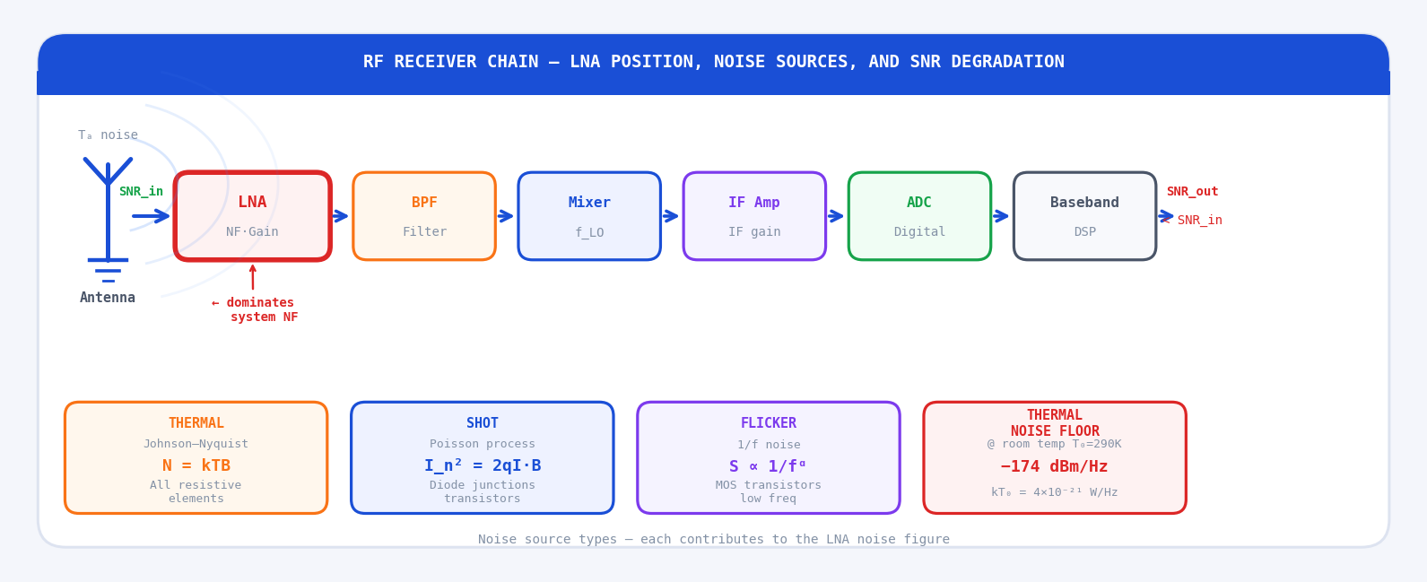
The LNA is always the first active component in an RF receive chain. It sits directly after the antenna (and any unavoidable passive components such as filters, switches, or duplexers). Its job is to bring the received signal up to a level where subsequent stages — mixers, IF amplifiers, ADCs — can process it, without the LNA's own noise drowning out the wanted signal in the process.

Applications

LNAs appear in virtually every system that needs to detect weak RF signals:

Wireless communications (5G, Wi-Fi, LTE). Base station receivers and handset chips both contain LNAs in their receive front ends. 5G mmWave receivers at 28 GHz and 39 GHz require LNAs with NF below 4 dB despite operating at frequencies where transistor performance degrades. Wi-Fi 6E (6 GHz) receivers integrate LNAs with NF of 2–3 dB in SoC silicon.
Radar systems. Both pulsed and continuous-wave radars rely on LNAs to detect target echoes that can be 120 dB or more below the transmitted pulse. The LNA's noise figure directly limits the minimum detectable radar cross-section and therefore the maximum detection range.
Satellite communications and GNSS. Satellite signals arrive at Earth with path losses exceeding 180 dB. GPS L1 signals at −130 dBm are recovered only because sensitive LNA front ends (often with NF < 1 dB) are used, frequently tower-mounted to eliminate cable loss before amplification.
RF sensing and IoT. Long-range IoT protocols such as LoRa, Sigfox, and NB-IoT require receiver sensitivities of −130 dBm or better. LNAs with NF of 1.5–2.5 dB operating at currents as low as 1–5 mA are now available in tiny packages for battery-constrained sensor nodes.
Radio astronomy and scientific instruments. Radio telescopes use cryogenically cooled LNAs (operating at 4–15 K) achieving NF below 0.1 dB — equivalent noise temperatures below 7 K. These represent the state of the art in low-noise amplification.

📌 LNA vs General-Purpose Amplifier — The Key Distinction

A general RF amplifier optimises for gain, output power, or bandwidth. An LNA optimises specifically for noise figure, accepting compromises in gain flatness, output power, or even input match if they result in lower NF. The entire transistor bias point, topology choice, input matching network, and PCB layout are driven by the question: how little noise can this design add to the signal?

Receiver Chain Context

Typical RF Receiver Architecture

A superheterodyne receiver — by far the most common architecture — processes signals in the following sequence:

Fig 2 — Superheterodyne receiver chain with key function of each stage

Each stage in this chain has a distinct role. The BPF after the LNA selects the desired band and rejects out-of-band interference before the mixer. The mixer translates the RF signal down to an intermediate frequency (IF) using a local oscillator (LO). The IF filter rejects the image frequency and adjacent channels. The IF amplifier provides most of the receiver's variable gain (AGC). The ADC digitises the signal for software-defined processing.

Importance of Placing the LNA Close to the Antenna

Any passive component between the antenna and the LNA — a cable, a connector, a filter, an RF switch, a duplexer — has an insertion loss L > 0 dB. At room temperature, a passive lossy element has a noise figure equal to its loss in dB. This means every decibel of loss before the LNA adds exactly one decibel to the system noise figure, degrading receiver sensitivity equally.

This is why tower-mounted LNAs (TMLNAs) are used in base stations: the LNA is mounted at the antenna, amplifying the signal before it travels down the long coaxial feeder to the base station equipment. A 3 dB feeder loss that previously degraded the system NF by 3 dB now appears after the LNA and its contribution is divided by the LNA gain — typically 20 dB (100×). Its effective NF contribution drops from 3 dB to just 0.03 dB.

Impact of LNA on Overall System Sensitivity

Receiver sensitivity — the minimum signal power the receiver can detect — is directly determined by the system noise figure. For a given modulation scheme requiring minimum SNR of SNR_min:

Receiver sensitivity

P_{min} = - 174 + 10 {log}_{10} (B) + {NF}_{sys} + {SNR}_{min} dBm

B is the receiver noise bandwidth in Hz. −174 dBm/Hz is the thermal noise floor at T₀ = 290 K. Every 1 dB improvement in NF_sys improves sensitivity by 1 dB — the link range increases by 12%.

Improving NF_sys by 1 dB improves sensitivity by 1 dB, which in a free-space link (where path loss ∝ R²) extends the maximum link range by a factor of 10^(1/20) ≈ 1.12 — a 12% range increase for every 1 dB of NF improvement. In a 2-path or urban propagation environment (path loss ∝ R⁴) the gain is even larger: 10^(1/40) per 1 dB NF — compounding across an entire network.

Noise Fundamentals

The Three Fundamental Noise Types

Noise in electronic components arises from physical phenomena at the microscopic level. Three types are relevant to LNA design:

Thermal Noise (Johnson–Nyquist Noise)

Thermal noise is generated by the random thermal motion of electrons in any resistive element at a temperature above absolute zero. It is present in every resistor, every transistor channel, every transmission line, and every antenna. The available noise power from a resistor R at temperature T in bandwidth B is independent of the resistance value:

Available thermal noise power

N = k T B W

k = 1.381 × 10⁻²³ J/K (Boltzmann's constant). T = absolute temperature in kelvin. B = noise bandwidth in Hz. This is the fundamental lower limit of noise — it cannot be reduced without reducing temperature or bandwidth.

The associated noise voltage (open-circuit) across the resistor is:

Open-circuit thermal noise voltage (rms)

v_{n} = \sqrt{4 k T R B} V

For R = 50 Ω at T = 290 K in B = 1 Hz: v_n = √(4 × 1.381×10⁻²³ × 290 × 50) = 0.895 nV/√Hz. The spectral density is v_n/√B = √(4kTR) V/√Hz.

Shot Noise

Shot noise arises from the discrete, quantised nature of electric charge. When charge carriers (electrons or holes) cross a potential barrier — such as a p-n junction in a transistor — they do so in random, independent events. The resulting current fluctuations have a flat (white) power spectral density:

Shot noise current spectral density

i_{n}^{2} = 2 q I B A²

q = 1.602 × 10⁻¹⁹ C (electron charge). I = DC bias current in amperes. B = bandwidth in Hz. Shot noise dominates in bipolar transistors and diodes at RF frequencies.

Flicker Noise (1/f Noise)

Flicker noise has a power spectral density that falls with frequency approximately as 1/f, hence the name. It dominates at low frequencies (below a few MHz in most transistors) and is caused by trapping and release of carriers at defect sites in the semiconductor lattice. In MOSFET transistors — the dominant technology in integrated LNAs — flicker noise can extend to higher frequencies than in bipolar devices, and is characterised by the corner frequency f_c above which thermal noise dominates:

Flicker noise voltage spectral density

S_{v}^{} (f) = \frac{K}{C_{ox} W L f} V²/Hz

K is a process-dependent constant. C_ox is oxide capacitance per unit area. W and L are transistor width and length. Longer channel transistors (larger WL) have lower flicker noise — an important design trade-off in low-frequency LNAs.

📌 Which Noise Type Matters for LNA Design?

At RF frequencies (above ~100 MHz), thermal noise dominates in both the source impedance and in the transistor channel resistance. Shot noise is the main mechanism in bipolar transistors. Flicker noise is generally below the corner frequency and can usually be neglected for the LNA noise figure calculation at RF — though it matters for oscillator phase noise and direct-conversion receiver DC offset.

Thermal Noise Power Density and the −174 dBm/Hz Floor

At the standard reference temperature T₀ = 290 K (approximately room temperature, 17°C), the available thermal noise power spectral density — the noise power per unit bandwidth — is:

Thermal noise power spectral density at T₀ = 290 K

\frac{N}{B} = k T_{0} = 1.381 \times 10^{- 23} \times 290 = 4.00 \times 10^{- 21} W/Hz

Converting to dBm/Hz: 10 log₁₀(4.00×10⁻²¹ / 10⁻³) = 10 log₁₀(4.00×10⁻¹⁸) = −173.98 ≈ −174 dBm/Hz.

This value of −174 dBm/Hz is the absolute lower limit of noise power that any passive component at room temperature and any receiver built from such components can achieve. It is the universal baseline from which all receiver sensitivity calculations start.

For any finite bandwidth B, the total available noise power is:

Total noise power in bandwidth B

N_{total} = - 174 + 10 {log}_{10} (B) dBm

For B = 1 MHz: N = −174 + 60 = −114 dBm. For B = 20 MHz (Wi-Fi): N = −174 + 73 = −101 dBm. For B = 200 MHz (5G NR): N = −174 + 83 = −91 dBm. Wider bandwidth → higher noise floor → lower sensitivity.

Signal-to-Noise Ratio (SNR)

The Signal-to-Noise Ratio is the ratio of wanted signal power S to noise power N at the same point in the signal chain, expressed in dB:

Signal-to-noise ratio

SNR = 10 {log}_{10} \frac{S}{N} dB

Both S and N in watts (or both in milliwatts). SNR in dB can also be computed as S(dBm) − N(dBm). For reliable demodulation: BPSK needs SNR ≥ 10 dB, 16-QAM needs ≥ 18 dB, 64-QAM needs ≥ 25 dB, 256-QAM needs ≥ 31 dB.

As a signal passes through an amplifier that adds noise, the output SNR is always less than the input SNR — the signal and the amplifier's noise are both present at the output, and the noise has grown relative to the signal. Quantifying exactly how much SNR is lost through an amplifier is the purpose of the noise figure.

Noise Figure — The Core Concept

Definition: NF = SNR_in / SNR_out

The noise figure of a two-port device is defined as the ratio of input SNR to output SNR, measured in dB. The input SNR is the SNR of the signal at the device's input port; the output SNR is the SNR at the output port. Both are measured with the source at the standard reference temperature T₀ = 290 K:

Noise figure definition

NF = 10 {log}_{10} (\frac{{SNR}_{in}}{{SNR}_{out}}) dB

NF ≥ 0 dB always. NF = 0 dB means a perfectly noiseless amplifier — the SNR is unchanged. Every real amplifier has NF > 0 dB. The source noise (kT₀B) is included in both SNR_in and SNR_out, so NF measures only the amplifier's added noise.

Noise Factor F and the Conversion to NF

The linear (non-dB) equivalent is the noise factor F:

Noise factor F (linear) — relationship to NF

F = \frac{{SNR}_{in}}{{SNR}_{out}} = 10^{\frac{NF}{10}} NF = 10 {log}_{10} (F)

F ≥ 1 always. F = 1 (NF = 0 dB) is ideal. F = 2 (NF = 3.01 dB) means the output SNR is half the input SNR. The Friis cascade formula uses F (not NF) — always convert to linear before applying it.

An alternative expression defines F as the ratio of total output noise power to the output noise power due to the source alone:

Noise factor in terms of added noise

F = \frac{N_{out}}{G \cdot N_{source}} = 1 + \frac{N_{added}}{G \cdot k T_{0} B}

N_added is the noise power added by the amplifier itself, referred to the input. G is the amplifier's power gain. N_source = kT₀B is the source noise power. This form makes clear that F = 1 only if the amplifier adds zero noise.

Physical Meaning of NF

An LNA with NF = 1.5 dB means that the output SNR is 1.5 dB worse than the input SNR. Put differently: if a −90 dBm signal arrives at the antenna with an input SNR of 20 dB (noise floor at −110 dBm), the LNA's output will have an SNR of only 18.5 dB. The 1.5 dB is gone permanently — no subsequent processing can recover it.

This is why every decibel of NF improvement in the LNA translates directly into the same improvement in receiver sensitivity and ultimately link range.

Typical LNA NF Values

Application	Frequency	Typical NF	Technology
Radio astronomy	1–10 GHz	< 0.1 dB	Cryo-cooled HEMT (4–15 K)
Satellite ground station	3.5–12 GHz	0.3 – 0.8 dB	GaAs pHEMT
GPS / GNSS receiver	1.2 – 1.6 GHz	0.7 – 1.2 dB	SiGe BiCMOS or GaAs
Cellular base station	0.7 – 3.5 GHz	0.8 – 1.5 dB	GaAs or SiGe
Wi-Fi / consumer	2.4 – 6 GHz	1.5 – 2.5 dB	CMOS or SiGe BiCMOS
5G mmWave	24 – 39 GHz	2.0 – 4.0 dB	CMOS 28 nm or GaAs
IoT / LoRa node	433 – 915 MHz	1.5 – 3.0 dB	CMOS (low power priority)

Measurement Techniques

Two methods dominate practical NF measurement. The Y-factor method uses a calibrated noise source switched between a hot state (T_hot, excess noise ratio known) and a cold state (T_cold = T₀). The ratio of output power in both states — the Y-factor — directly yields the noise factor:

Y-factor method — noise factor from hot/cold power ratio

F = \frac{T_{hot} / T_{0} - Y \cdot T_{cold} / T_{0}}{Y - 1} Y = \frac{P_{hot}}{P_{cold}}

With T_cold = T₀: F = (ENR_linear − Y + 1)/(Y − 1), where ENR = (T_hot − T₀)/T₀. This is automated in modern noise figure analysers and VNAs with noise figure option.

The cold-source method uses a calibrated vector network analyser to measure S-parameters and noise wave parameters, allowing NF measurement without a dedicated noise source — increasingly popular for on-wafer and mmWave measurements where calibrated noise sources are difficult to implement.

The Friis Formula for Cascaded Systems

Why the LNA Dominates System Noise

Consider a signal passing through a chain of amplifiers and passive elements. Each stage adds its own noise on top of the accumulated signal-plus-noise from previous stages. The total system noise factor, referred back to the system input, is given by the Friis noise formula:

Friis cascaded noise factor formula

F_{total} = F_{1} + \frac{F_{2} - 1}{G_{1}} + \frac{F_{3} - 1}{G_{1} G_{2}} + \frac{F_{4} - 1}{G_{1} G_{2} G_{3}} + \dots

All F values are linear (not dB). All G values are linear power gains (not dB). Convert: F = 10^(NF/10), G = 10^(G_dB/10) before applying the formula.

The structure of this formula reveals everything about why LNA design matters so much:

F₁ appears undivided. The noise factor of the first stage contributes directly to F_total — there is no gain preceding it to suppress its contribution. Every tenth of a dB in the LNA NF translates directly into system NF.
F₂ is divided by G₁. If the LNA provides G₁ = 20 dB (factor 100), then the second stage's noise contribution is reduced 100-fold. A mixer with F₂ = 8 dB (factor 6.3) contributes only (6.3−1)/100 = 0.053 to F_total — just 0.22 dB.
F₃ is divided by G₁·G₂, and so on. With sufficient first-stage gain, the entire receive chain's noise performance is determined almost entirely by the LNA.

💡 The Pre-LNA Loss Rule

If a passive element with loss L (linear, ≥ 1) precedes the LNA, it contributes F₁ = L to the cascade. Its gain is G₁ = 1/L. The LNA then becomes stage 2, with its noise contribution divided by G₁ = 1/L — meaning the LNA noise is multiplied by L. A 2 dB filter before the LNA effectively adds 2 dB to the LNA's NF as seen by the system. Place all passive components after the LNA whenever possible. When a filter must precede the LNA (e.g., for out-of-band rejection before a strong interferer compresses the LNA), choose the filter with the lowest possible insertion loss.

Design Insight: First Stage Gain and NF Are Critical

The Friis formula quantifies a fundamental design trade-off. To minimise F_total:

Minimise F₁ (LNA noise factor) — use the best available transistor and operate near its NF_min.
Maximise G₁ (LNA gain) — but not without limit. Higher gain increases the signal level at the LNA output, which the subsequent mixer must handle linearly. If the LNA gain is too high, a strong out-of-band interferer will compress the mixer. Gain control or a switchable attenuator (gain state switching) is often added for high-interference environments.
The optimum LNA gain is the minimum gain that makes the cascade NF insensitive to subsequent stages' noise — typically 15–20 dB is sufficient for most receiver chains.

Gain Concepts

Power Gain Definitions

Three distinct power gain definitions appear in LNA and amplifier literature. They differ in how they treat impedance mismatch at the input and output ports:

Transducer Power Gain (G_T)

Transducer gain is the ratio of power delivered to the load to the available power from the source — the maximum power the source can deliver to any load. It accounts for mismatch at both ports:

Transducer power gain

G_{T} = \frac{P_{load}}{P_{avs}} = \frac{| S_{21} |^{2} (1 - {| Γ_{s} |}^{2}) (1 - {| Γ_{L} |}^{2})}{{| 1 - S_{11} Γ_{s} |}^{2} {| 1 - Γ_{out} Γ_{L} |}^{2}}

G_T is what a signal analyser measures when the device is connected between a 50 Ω source and 50 Ω load. If both ports are matched (Γ_s = Γ_L = 0): G_T = |S21|². This is the gain reported in most datasheets.

Available Power Gain (G_A)

Available gain is the ratio of the amplifier's available output power to the available input power from the source. It depends only on source impedance, not on load impedance. It is the gain relevant to noise figure analysis — noise figure is defined with respect to available power:

Available power gain

G_{A} = \frac{P_{avo}}{P_{avs}} = \frac{| S_{21} |^{2} (1 - {| Γ_{s} |}^{2})}{{| 1 - S_{11} Γ_{s} |}^{2} (1 - {| Γ_{out} |}^{2})}

G_A is used in noise circle design. Constant G_A circles on the Smith chart (as a function of Γ_s) are the gain circles plotted alongside noise circles to find the best operating point.

Operating Power Gain (G_P)

Operating gain is the ratio of power delivered to the load to the power actually delivered to the amplifier's input port. It depends on load impedance but not on source impedance:

Operating power gain

G_{P} = \frac{P_{load}}{P_{in}} = \frac{| S_{21} |^{2} (1 - {| Γ_{L} |}^{2})}{(1 - {| S_{11} |}^{2}) {| 1 - Γ_{out} Γ_{L} |}^{2}}

G_P is useful for power amplifier design where the input power delivered by the driver stage is known. For LNAs, G_T and G_A are more commonly used.

S-Parameters: S21 as the Forward Gain

In the context of a 50 Ω system (source and load both at Z₀ = 50 Ω), the transducer gain simplifies to |S21|². The scattering parameter S21 is the complex forward transmission coefficient — the ratio of the wave leaving port 2 to the wave entering port 1 when port 2 is terminated in Z₀:

Gain from S21 in a matched 50 Ω system

G_{T,dB} = 20 {log}_{10} | S_{21} | = 10 {log}_{10} {| S_{21} |}^{2}

|S21| is a voltage ratio (hence 20 log), but |S21|² is a power ratio (hence 10 log) — both give the same dB result. An LNA with |S21| = 10 → 20 log(10) = 20 dB gain.

Input Matching vs Noise Matching

Conjugate Matching for Maximum Gain

Maximum power transfer from source to amplifier input requires conjugate matching: the source impedance Z_s must equal the complex conjugate of the amplifier's input impedance Z_in*. In terms of reflection coefficients, the optimum source reflection coefficient for maximum gain is:

Optimum source reflection coefficient for maximum gain

Γ_{s, conj} = Γ_{in}^{*} = (S_{11} + \frac{S_{12} S_{21} Γ_{L}}{1 - S_{22} Γ_{L}})^{*}

For a unilateral approximation (S12 ≈ 0), Γ_s,conj ≈ S11*. The matching network is designed to transform the 50 Ω source to present Γ_s,conj to the transistor input. This maximises gain but does not minimise NF.

Noise Matching for Minimum NF

The noise figure of a transistor is minimised when the source reflection coefficient equals the optimum noise reflection coefficient Γ_opt — a quantity that is a fundamental property of the transistor at a given bias point and frequency. Γ_opt is measured as part of the transistor's four noise parameters:

Noise figure as a function of source reflection coefficient

NF = {NF}_{\min} + \frac{4 R_{n} {| Γ_{s} - Γ_{opt} |}^{2}}{Z_{0} (1 - {| Γ_{s} |}^{2}) {| 1 + Γ_{opt} |}^{2}}

NF = NF_min only when Γ_s = Γ_opt exactly. R_n (noise resistance) controls how fast NF increases as Γ_s moves away from Γ_opt. A smaller R_n means the design is more tolerant of matching errors.

The Gain–Noise Trade-off and Source Reflection Coefficient

The fundamental problem is that Γ_opt and Γ_s,conj* are generally not equal. The point that gives minimum NF and the point that gives maximum gain are different points on the Smith chart. The LNA designer must choose a source impedance that balances the two requirements:

Fig 3 — Conceptual Smith chart showing noise circles (NF contours) and gain circles. The optimum design point lies between Γ_opt and Γ_s,conj.

Noise circles are centred at Γ_opt. Gain circles are centred near Γ*_in. The design point is chosen on an acceptable noise circle that intersects a satisfactory gain circle — typically accepting 0.5–2 dB of gain loss to operate close to NF_min.

The practical resolution of this trade-off depends on the application priority:

Sensitivity-limited receivers (satellite, GNSS, radio astronomy): operate as close to Γ_opt as possible. Accept gain reduction. Use an output matching network to maximise power transfer to the next stage independently of the input match.
Gain-limited systems (active arrays, short-range links): operate closer to the conjugate match. Accept the slightly degraded NF.
Simultaneous noise and power matching (SNPM): when Γ_opt ≈ Γ*_in — which can be engineered in an inductively degenerated LNA topology — both conditions are satisfied at the same source impedance. This is the elegance of the inductive degeneration technique.

📌 What Comes Next

This article has established the context and noise fundamentals. Part 2 of this series covers the practical LNA parameters in detail — linearity (IIP3, P1dB, dynamic range), stability (Rollett K-factor, stability circles), S-parameter characterisation, and the noise parameters NF_min, R_n, and Γ_opt in the context of real device selection. Part 3 covers LNA circuit topologies, bias networks, PCB layout, and worked design examples.

Questions & Worked Examples

Work through each problem fully before reading the solution.

01

Thermal Noise Power and Noise Voltage

Problem: A 50 Ω antenna at T = 290 K feeds a 5G NR receiver with 100 MHz bandwidth. (a) What is the available thermal noise power at the antenna output in watts and dBm? (b) What is the open-circuit noise voltage spectral density? (c) If the received signal power is −90 dBm, what is the input SNR?

(a) Available thermal noise power

N = k T B = 1.381 \times 10^{- 23} \times 290 \times 10^{8} = 4.0 \times 10^{- 13} W

Convert to dBm

N = - 174 + 10 {log}_{10} (10^{8}) = - 174 + 80 = - 94 dBm

(b) Open-circuit noise voltage spectral density

\frac{v_{n}}{\sqrt{B}} = \sqrt{4 k T R} = \sqrt{4 \times 1.381 \times 10^{- 23} \times 290 \times 50} = 0.895 nV/√Hz

SNR = P_{s} - N = - 90 - (- 94) = + 4 dB

Answer: N = 4.0×10⁻¹³ W = −94 dBm | v_n/√B = 0.895 nV/√Hz | SNR_in = 4 dB

An SNR of only 4 dB at the antenna means the signal is barely above the noise floor — this is typical for cell-edge 5G NR. Even a tiny amount of additional noise from the LNA (say NF = 2 dB) would reduce the receiver SNR to 4 − 2 = 2 dB, which is below the minimum SNR for QPSK (SNR_min ≈ 6 dB). This illustrates why 5G base station LNAs must achieve NF ≤ 1.5 dB, and why every tenth of a dB matters at the cell edge.

02

Converting Between NF, Noise Factor, and Noise Temperature

Problem: Three LNAs are specified with the following noise performance. Convert each to all three representations (NF in dB, noise factor F, equivalent noise temperature T_e at T₀ = 290 K): (a) LNA-X: NF = 0.8 dB (b) LNA-Y: F = 1.50 (c) LNA-Z: T_e = 120 K

(a) LNA-X: NF = 0.8 dB → F and T_e

F = 10^{\frac{0.8}{10}} = 1.202 T_{e} = (1.202 - 1) \times 290 = 58.5 K

(b) LNA-Y: F = 1.50 → NF and T_e

NF = 10 {log}_{10} (1.50) = 1.76 dB T_{e} = 0.50 \times 290 = 145 K

F = 1 + \frac{120}{290} = 1.414 NF = 10 {log}_{10} (1.414) = 1.50 dB

Summary: LNA-X: F=1.202, T_e=58.5 K | LNA-Y: NF=1.76 dB, T_e=145 K | LNA-Z: F=1.414, NF=1.50 dB

These conversions must be fluent — the Friis formula uses F (linear), datasheets specify NF (dB), and satellite/radio astronomy work uses T_e (kelvin). LNA-X with T_e = 58.5 K is excellent — typical of a high-quality GaAs pHEMT at 2 GHz. LNA-Z at T_e = 120 K (NF = 1.5 dB) is a solid mid-range performer. LNA-Y at 1.76 dB is reasonable for a consumer-grade CMOS device but would be inadequate for a satellite application.

03

Friis Cascade — Tower-Mounted vs Base-Station LNA

Problem: A cellular base station has a 3 dB coaxial feeder loss between antenna and receiver, followed by an LNA with NF = 1.0 dB and gain = 20 dB, then a mixer with NF = 9 dB. Compare the system NF for two configurations: (A) LNA at the base station (after the cable), and (B) LNA tower-mounted at the antenna (before the cable). The cable loss is the same in both cases.

Configuration A — Cable → LNA → Mixer (base station LNA)

F_{A} = 2.0 + \frac{1.259 - 1}{0.5} + \frac{7.943 - 1}{0.5 \times 100} = 2.0 + 0.518 + 0.139 = 2.657

Cable: F₁ = 10^(3/10) = 2.0, G₁ = 0.5. LNA: F₂ = 10^(1.0/10) = 1.259, G₂ = 100. Mixer: F₃ = 10^(9/10) = 7.943.

NF_sys for Configuration A

{NF}_{A} = 10 {log}_{10} (2.657) = 4.24 dB

Configuration B — LNA → Cable → Mixer (tower-mounted LNA)

F_{B} = 1.259 + \frac{2.0 - 1}{100} + \frac{7.943 - 1}{100 \times 0.5} = 1.259 + 0.010 + 0.139 = 1.408

NF_sys for Configuration B

{NF}_{B} = 10 {log}_{10} (1.408) = 1.49 dB

Config A (base station LNA): NF_sys = 4.24 dB | Config B (tower-mounted LNA): NF_sys = 1.49 dB

Moving the LNA from the base station to the tower improves system NF by 2.75 dB — a dramatic improvement from a trivial physical rearrangement. In a free-space link this extends the maximum range by 10^(2.75/20) ≈ 1.37, or 37%. In a real cellular network with shadowing exponent n = 3.5 the range extension is 10^(2.75/35) ≈ 1.20, or 20% — still highly significant. This explains why virtually every modern cellular base station uses a tower-mounted pre-amplifier.

04

Gain and NF — Three Power Gain Definitions Applied

Problem: An LNA has S-parameters at 2.4 GHz: S11 = 0.35∠−60°, S21 = 5.0∠120°, S12 = 0.05∠30°, S22 = 0.20∠−45°. The source reflection coefficient is Γ_s = 0.2∠45° and the load is 50 Ω (Γ_L = 0). Calculate: (a) transducer gain G_T in dB, (b) confirm S21 gives the correct gain in a matched 50 Ω system (Γ_s = Γ_L = 0).

(a) G_T with Γ_s = 0.2∠45°, Γ_L = 0

G_{T} = \frac{{| S_{21} |}^{2} (1 - {| Γ_{s} |}^{2}) (1 - {| Γ_{L} |}^{2})}{{| 1 - S_{11} Γ_{s} |}^{2} {| 1 - Γ_{out} Γ_{L} |}^{2}}

With Γ_L = 0: Γ_out = S22, the denominator second factor = 1

G_{T} = \frac{25 \times (1 - 0.04) \times 1}{{| 1 - 0.35 ∠ - 60° \times 0.2 ∠ 45° |}^{2}}

S11·Γ_s = 0.35×0.2 ∠(−60°+45°) = 0.07∠−15° → 1 − 0.07∠−15° ≈ 0.932∠0.64° → |…|² ≈ 0.869

G_{T} = \frac{25 \times 0.96}{0.869} = 27.6 \to 14.4 dB

(b) Matched 50 Ω case: Γ_s = Γ_L = 0 → G_T = |S21|²

G_{T} = {| S_{21} |}^{2} = {5.0}^{2} = 25 \to 10 {log}_{10} (25) = 13.98 \approx 14.0 dB

When Γ_s = Γ_L = 0 (both ports terminated in exactly 50 Ω), G_T = |S21|² exactly. The slight difference (14.4 vs 14.0 dB) in part (a) arises because Γ_s ≠ 0 — the mismatch at the source slightly increases gain via the (1−|Γ_s|²)/|1−S11Γ_s|² factor.

Answer: G_T = 14.4 dB with Γ_s = 0.2∠45° | G_T = 14.0 dB in matched 50 Ω system

The 0.4 dB difference confirms that the source mismatch (Γ_s = 0.2) changes the transducer gain — in this case slightly increasing it because the source is not presenting the conjugate match but is favourably positioned. In practice, datasheet gain is always measured with Γ_s = Γ_L = 0 (50 Ω), so the in-circuit gain may differ from the datasheet value once matching networks are added.