How Standing Waves Form
In Part 3 we found that a mismatched load sends back a reflected wave V⁻ = Γ·V⁺. Both waves exist on the line at the same time and the same frequency, travelling in opposite directions. At some points they arrive in phase and add; at others they arrive out of phase and partly cancel. Because the two waves move in opposite directions, these points stay fixed along the line — a standing wave.
Fig 1 shows the three regimes. A matched line has a flat voltage profile. A total reflection (short, open or pure reactance) produces true nulls where the voltage is zero and peaks of twice the incident voltage. Anything in between produces a ripple whose depth grows with |Γ|.
Voltage Maxima and Minima
- Spacing. Max to max = λ/2; max to adjacent min = λ/4.
- Load position. For a resistive load R > Z₀ (θ = 0°) there is a voltage maximum right at the load. For R < Z₀ (θ = 180°) there is a minimum at the load. A short has a null at the load, an open has a peak.
- Current. The current standing wave is the mirror image: current maxima sit at voltage minima. At a voltage maximum the line looks like a high resistance Z₀·VSWR; at a minimum, a low resistance Z₀/VSWR.
Definition of VSWR
The voltage standing wave ratio is the ratio of the maximum to the minimum voltage magnitude along a line: VSWR = V_max / V_min. It is written as a ratio, e.g. "1.5 : 1", and ranges from 1 (perfect match) to ∞ (total reflection).
For a purely resistive load the VSWR is simply the ratio of the larger to the smaller resistance: R/Z₀ if R > Z₀, or Z₀/R if R < Z₀. A 100 Ω or a 25 Ω load on 50 Ω both give VSWR 2 : 1.
VSWR, Return Loss and Mismatch Loss
| VSWR | |Γ| | Return loss | Power reflected | Mismatch loss | Typical meaning |
|---|---|---|---|---|---|
| 1.0 : 1 | 0 | ∞ | 0% | 0 dB | Perfect match |
| 1.2 : 1 | 0.091 | 20.8 dB | 0.8% | 0.036 dB | Excellent (test equipment, filters) |
| 1.5 : 1 | 0.200 | 14.0 dB | 4.0% | 0.18 dB | Very good antenna match |
| 1.92 : 1 | 0.316 | 10.0 dB | 10% | 0.46 dB | Common antenna bandwidth limit |
| 2.0 : 1 | 0.333 | 9.54 dB | 11.1% | 0.51 dB | Acceptable for many radios |
| 3.0 : 1 | 0.500 | 6.02 dB | 25% | 1.25 dB | Poor; many transmitters fold back power |
| 5.0 : 1 | 0.667 | 3.52 dB | 44% | 2.55 dB | Badly mismatched |
VSWR on the Smith Chart
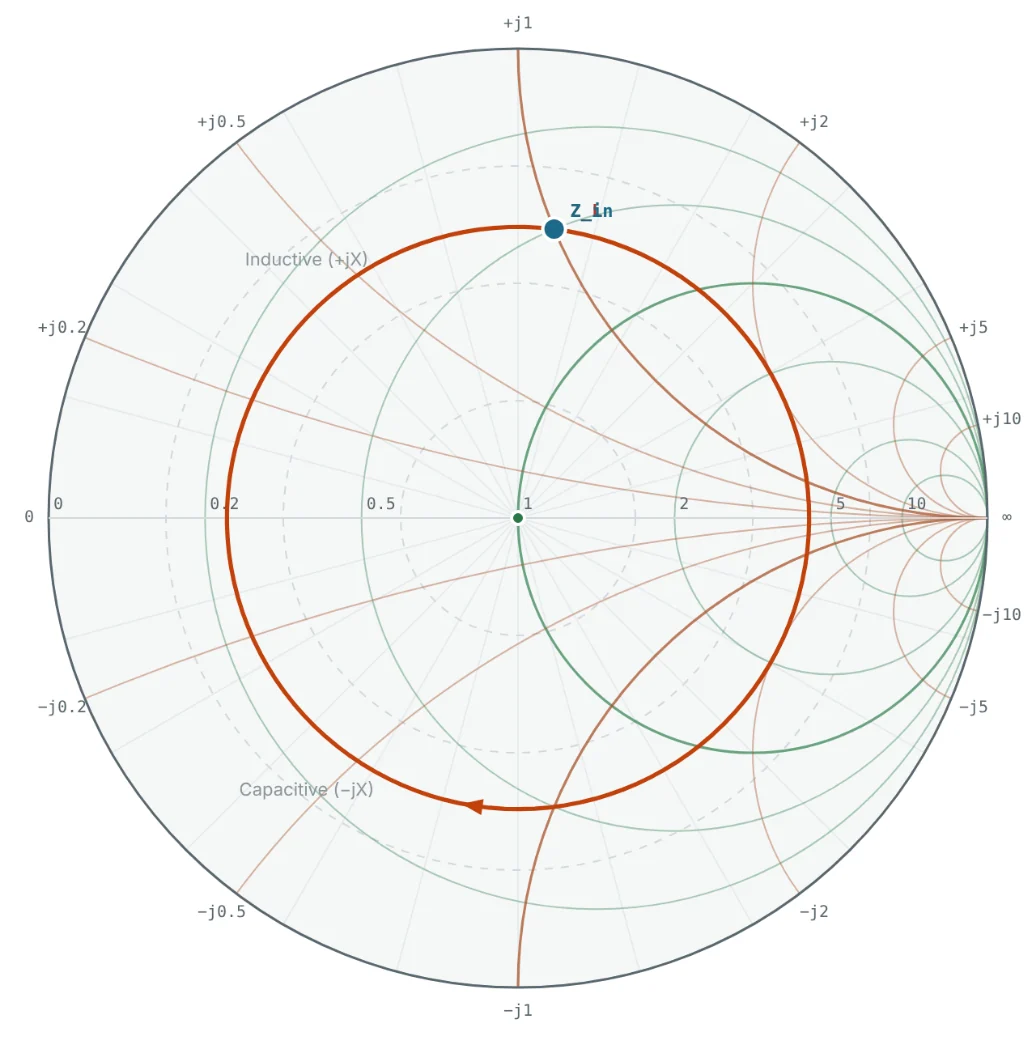
On a lossless line, moving along the line changes only the phase of Γ, never its magnitude. Every impedance seen along the line therefore lies on a circle of constant |Γ| centred on the chart — the VSWR circle. The circle crosses the right-hand real axis at r = VSWR (the voltage maximum) and the left-hand real axis at r = 1/VSWR (the voltage minimum). This gives a quick graphical way to read VSWR: draw the circle through the load and read where it hits the right half of the real axis.

Why VSWR Matters
- Transmitter safety. High VSWR puts voltage peaks of up to (1 + |Γ|) × the incident voltage on the line and output stage. Power amplifiers reduce output or shut down above a VSWR limit, often 2 : 1 or 3 : 1.
- Delivered power. Mismatch loss directly reduces the radiated or received power.
- Cable stress. Voltage and current peaks increase dielectric stress and conductor heating at fixed spots along the line.
- Frequency response. Reflections at both ends of a cable create ripple in gain versus frequency, with a period set by the cable length.
- Antenna bandwidth. Antenna bandwidth is commonly defined as the frequency range where VSWR ≤ 2 : 1 or S11 ≤ −10 dB (VSWR 1.92 : 1).
A lossy cable attenuates the reflected wave twice — on the way to the load and on the way back — so a VSWR meter at the transmitter reads better than the true antenna VSWR. Part 12 quantifies this effect.
Worked Examples
From Γ to VSWR and Return Loss
Problem: Find the VSWR, return loss and mismatch loss for |Γ| = 0.2, 1/3 and 0.5.
| |Γ| | VSWR = (1+|Γ|)/(1−|Γ|) | RL = −20 log|Γ| | ML = −10 log(1−|Γ|²) |
|---|---|---|---|
| 0.2 | 1.2/0.8 = 1.50 | 13.98 dB | 0.177 dB |
| 0.333 | 1.333/0.667 = 2.00 | 9.54 dB | 0.512 dB |
| 0.5 | 1.5/0.5 = 3.00 | 6.02 dB | 1.249 dB |
These three values match the 75 Ω, 100 Ω and 30 − j40 Ω loads of Parts 2 and 3.
Interpreting a VSWR Specification
Problem: An antenna datasheet promises VSWR ≤ 1.5 : 1. What fraction of power can be reflected at worst?
Reflected Power at VSWR 3 : 1
Problem: A 100 W transmitter drives a lossless line into a load with VSWR 3 : 1. How much power is reflected and how much reaches the load?
The 25 W returns to the transmitter, where — depending on its output impedance — it is re-reflected or dissipated as heat.
Peak and Minimum Line Voltage
Problem: The forward wave on a line has amplitude 10 V and the load is 100 Ω on 50 Ω (Γ = 1/3). Find V_max, V_min and where the first maximum occurs.
Because θ = 0° for a resistive load larger than Z₀, the peak sits right at the load — the blue curve in Fig 1.
Locating the Voltage Maximum for a Complex Load
Problem: For Z_L = 25 + j50 Ω (Γ = 0.620 ∠ 82.9°), how far from the load are the first voltage maximum and minimum?
On the Smith chart this is the clockwise rotation from z_L to the right-hand real axis, where the impedance is a pure 4.27 × 50 = 213 Ω. Part 5 uses exactly this idea for impedance transformation.
Summary
- Forward and reflected waves interfere to form a standing wave that repeats every λ/2.
- VSWR = V_max/V_min = (1 + |Γ|)/(1 − |Γ|); it ignores the phase of Γ.
- VSWR 2 : 1 ≈ 11% reflected and 0.5 dB mismatch loss; S11 = −10 dB corresponds to VSWR 1.92 : 1.
- On the Smith chart, a lossless line keeps the impedance on a constant-VSWR circle; it crosses the real axis at VSWR and 1/VSWR.
If the impedance changes as we move along the line, we can use the line itself to change impedance. Part 5: Impedance Transformation Along Transmission Lines explains how.
Put It Into Practice
Use the NEXT ANTENNAS calculators to apply the ideas from this article to real designs.