Why Impedance Matching Matters
Every RF system is built from interconnected blocks — antennas, cables, amplifiers, filters, mixers — each with its own input and output impedance. When those impedances disagree, power is reflected back toward the source rather than delivered to the load. In a transmitter this wastes power and can damage the PA. In a receiver it degrades SNR. In an antenna system it raises VSWR, narrows bandwidth, and radiates less efficiently.
Impedance matching is the engineering discipline of eliminating — or at least minimising — these reflections. The goal is always the same: present each port with the impedance it expects so that maximum power transfers across every interface.
RF systems almost universally use 50 Ω as the system impedance. It emerged historically as a compromise between the 75 Ω impedance of minimum-loss coaxial cable and the 30 Ω impedance of maximum-power-handling coax. Television and cable distribution systems use 75 Ω. Everything else — test equipment, connectors, PCB traces, antennas — is designed around 50 Ω.
Reflection Coefficient Γ
The reflection coefficient Γ (gamma) is the fundamental quantity describing how well two impedances are matched. It is defined as the ratio of the reflected wave amplitude to the incident wave amplitude at the interface:
Γ ranges from −1 to +1 in the real case, and has magnitude |Γ| between 0 and 1 in general. Three special cases are worth memorising:
- Perfect match: Z_L = Z_0 → Γ = 0. No reflection. All power delivered to load.
- Open circuit: Z_L = ∞ → Γ = +1. Full reflection, voltage doubling at the open.
- Short circuit: Z_L = 0 → Γ = −1. Full reflection, phase reversal, current doubling.
The reflected power fraction is |Γ|², and the transmitted power fraction is (1 − |Γ|²). A |Γ| of 0.1 means 1% of power is reflected — usually acceptable. A |Γ| of 0.5 means 25% of power is wasted — a serious mismatch.
VSWR — Voltage Standing Wave Ratio
When a reflected wave travels back toward the source and interferes with the incident wave, the superposition creates a standing wave pattern along the transmission line. The ratio of the voltage maximum to the voltage minimum in this pattern is the Voltage Standing Wave Ratio (VSWR):
VSWR is measured directly with a VSWR meter or a vector network analyser (VNA). It is an older metric than |Γ| but is still widely used in antenna and transmitter specifications because it is dimensionless, always ≥ 1, and easy to interpret:
- VSWR = 1.0:1 — Perfect match (theoretical ideal)
- VSWR = 1.5:1 — |Γ| = 0.20 — 4% reflected power — good for most applications
- VSWR = 2.0:1 — |Γ| = 0.33 — 11% reflected power — acceptable for many antennas
- VSWR = 3.0:1 — |Γ| = 0.50 — 25% reflected power — borderline, check PA tolerance
- VSWR > 3.0:1 — Significant mismatch — redesign the matching network
Return Loss
Return loss (RL) is the same information as |Γ|, expressed in dB. It is always a positive number — a higher return loss means less power is reflected, which is better:
The S11 parameter measured by a VNA is directly the return loss (with sign): S11 = 20·log₁₀(|Γ|), so S11 = −20 dB is the same as RL = 20 dB. In practice, an S11 below −10 dB (RL > 10 dB, |Γ| < 0.316, VSWR < 2.0) is considered the minimum acceptable match for most antenna applications.
All three describe the same mismatch. S11 is complex (gives phase too). |Γ| is its magnitude. Return loss is −20·log₁₀(|Γ|). VSWR is (1+|Γ|)/(1−|Γ|). A VNA plots S11; an antenna datasheet quotes VSWR; a filter spec quotes return loss. Know all three.
The Smith Chart
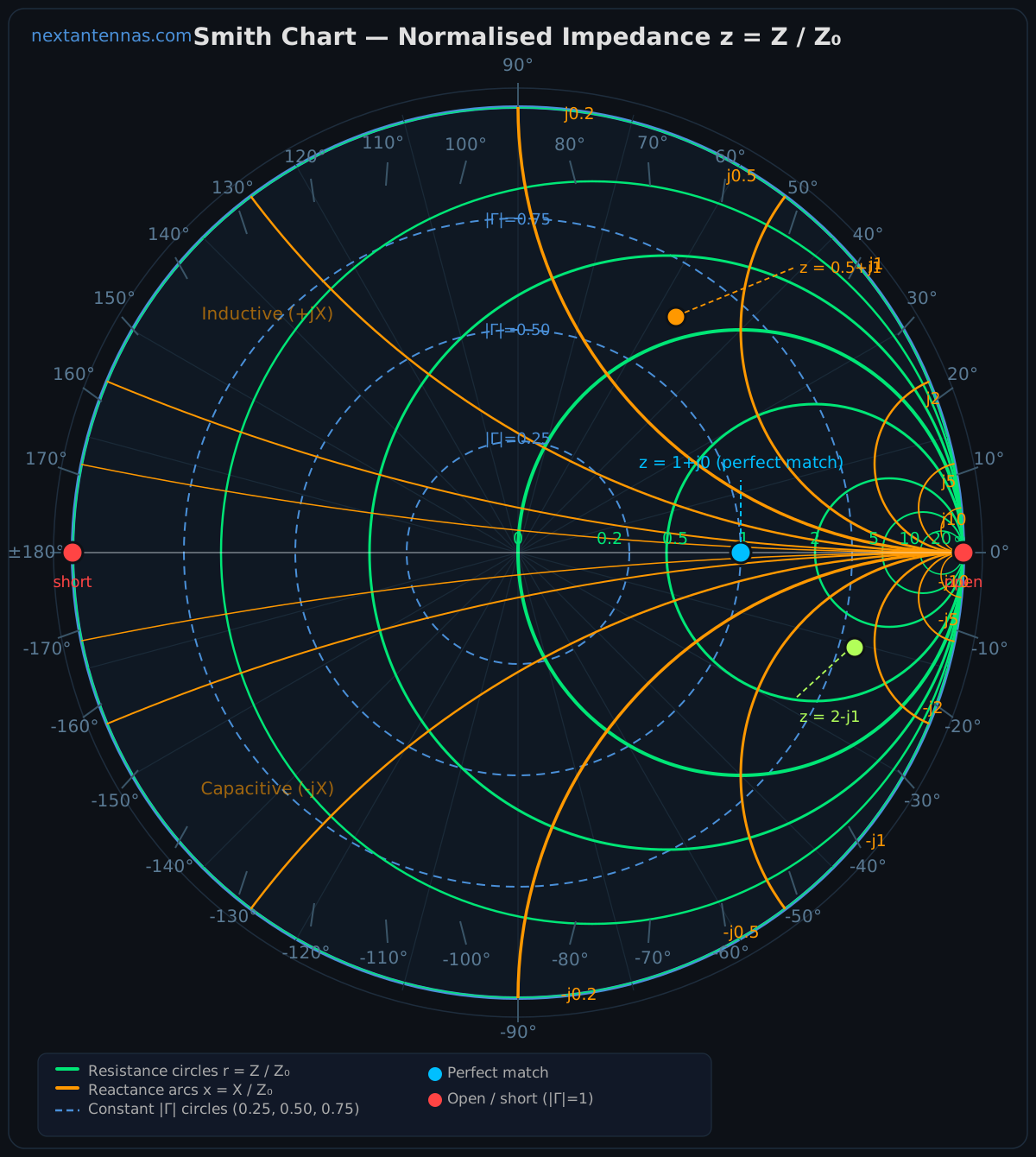
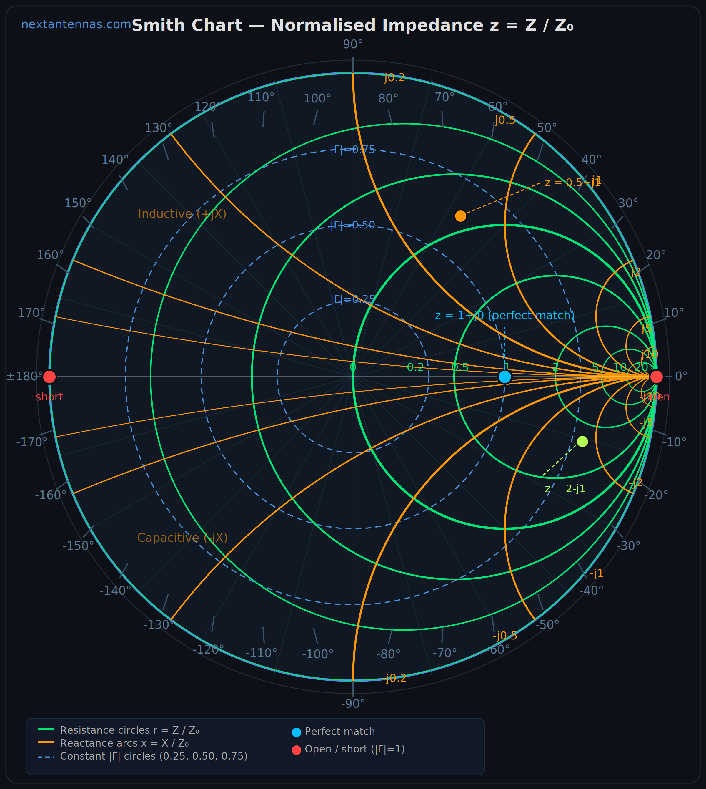
The Smith chart is a graphical tool for solving transmission line and impedance matching problems without complex algebra. Developed by Phillip H. Smith at Bell Labs in 1939, it maps the entire complex impedance plane onto a unit circle using the reflection coefficient as the underlying coordinate system.
The chart plots normalised impedance z = Z/Z₀ = r + jx, where r is the normalised resistance and x is the normalised reactance. The key features are:
- Resistance circles: constant-r circles, all tangent to the right edge of the chart. The centre of the chart is r = 1, x = 0 — the perfect match point (50 Ω for a 50 Ω system).
- Reactance arcs: constant-x arcs. Upper half = inductive (positive x). Lower half = capacitive (negative x).
- Outer edge: |Γ| = 1 — all points here are pure reactances (no resistance, total reflection).
- Centre: |Γ| = 0 — perfect match.
- Circles of constant |Γ|: concentric circles around the centre. Moving along a circle of constant radius means moving along a lossless transmission line — the impedance rotates around the chart as frequency or line length changes.
High-quality Smith chart for printing and reference. Available as a lossless vector SVG (scales to any size) or a 2400×2680 px PNG for presentations and documents.
Reading the Smith Chart
To use the chart, normalise your impedance: z = Z/Z₀. Plot the point. Read off the |Γ| circle it sits on. The distance from the centre is |Γ|. Moving toward the generator (source) rotates the point clockwise around a constant-|Γ| circle; moving toward the load rotates counterclockwise. One full revolution = λ/2 of transmission line.
Adding a series element (inductor or capacitor) moves the point along a resistance circle. Adding a shunt element moves it along a conductance circle (you switch to the admittance Smith chart, which is rotated 180°). Matching consists of moving Z_L to the centre of the chart through a sequence of such moves.
Our Smith Chart Visualiser lets you add series and shunt inductors, capacitors, and resistors between a 50 Ω source and any load — the impedance trace, S11, VSWR, and |Γ| all update in real time. A live circuit schematic shows the network as you build it.
L-Networks
The L-network is the simplest two-element impedance matching network. It uses one series element and one shunt element, arranged to transform one real impedance to another. The name comes from the L-shape of the circuit diagram.
For matching a source impedance R_S to a load impedance R_L where R_L > R_S, the series element goes on the source side and the shunt element goes on the load side (or vice versa — there are two topologies). The design equations involve the Q factor of the network:
The L-network has no free design parameter — Q is fixed once R_S and R_L are chosen. If you need to control bandwidth, use a π-network or T-network, which add a third element and allow Q to be set independently of the impedance ratio.
π and T Networks
The π-network (two shunt elements + one series element) and T-network (two series elements + one shunt element) are three-element matching networks that provide an additional degree of freedom — the designer can choose Q independently and then calculate element values. Higher Q gives a narrower bandwidth and more selectivity; lower Q gives broadband matching with less filtering. The element values are derived by treating the network as two back-to-back L-networks sharing an intermediate virtual impedance R_virtual = R_high / (1 + Q²).
Quarter-Wave Transformer
For matching two real (purely resistive) impedances at a single frequency, the quarter-wave transformer is the most elegant solution. A transmission line section of electrical length λ/4 transforms an impedance Z_L to an input impedance Z_in:
The quarter-wave transformer is inherently narrowband — it provides a perfect match only at the design frequency f₀ and degrades symmetrically on either side. For broader bandwidth, multiple cascaded quarter-wave sections can be used (Chebyshev or binomial taper), at the cost of length and complexity.
A practical example: matching a 50 Ω feed to a 200 Ω patch antenna edge impedance at 2.4 GHz on FR-4 (εeff ≈ 3.5):
Stub Matching
Stub matching uses one or more short sections of open-circuited or short-circuited transmission line — called stubs — connected in shunt or series with the main line to cancel the reactive part of the load impedance. It is particularly useful in microstrip designs where lumped components are impractical at microwave frequencies.
Single Stub Tuner
The single-stub tuner consists of two design parameters: the distance d from the load to the stub, and the length ℓ of the stub. The procedure is:
- Step 1: Find the distance d from the load such that the admittance on the main line is Y_in = Y₀ + jB (real part equals the system admittance Y₀ = 1/Z₀).
- Step 2: Choose the stub length ℓ such that the stub admittance Y_stub = −jB, cancelling the susceptance.
- Step 3: For a short-circuit stub: ℓ = (λ/2π)·arctan(−B/Y₀). For an open-circuit stub: ℓ = −(λ/2π)·arctan(Y₀/B).
The single-stub tuner always has two solutions (two valid values of d). The shorter solution is preferred for bandwidth. Open-circuit stubs are easier to fabricate in microstrip (no via required) but are slightly longer than their short-circuit equivalents.
Double Stub Tuner
The double-stub tuner places two stubs at fixed positions (typically λ/8 or 3λ/8 apart) and varies both stub lengths. It is used when the load position is fixed and the distance to the stub cannot be adjusted. The trade-off is that certain load impedances fall in a "forbidden region" where the double-stub cannot match — in practice, this affects loads with |Γ| close to 1 at certain phase angles.
Practical Techniques for Minimising Return Loss
Theory gives you the starting point. In practice, several additional considerations determine whether your design achieves the target S11 on the bench.
1. Calibrate Your VNA Properly
A VNA measures S11 at its port. Every connector, adapter, and cable between the VNA port and your DUT adds electrical length and loss — and the VNA measures all of it unless you calibrate them out. Always perform a full SOLT (Short-Open-Load-Thru) or equivalent calibration at the plane of your DUT. A 1 mm error in calibration reference plane shifts the S11 phase by roughly 7° at 10 GHz — enough to make a matched network look mismatched.
2. Account for Component Parasitics
At RF frequencies, lumped components are not ideal. A chip capacitor has series inductance (ESL) and resistance (ESR). A chip inductor has shunt capacitance and resistance. Above the self-resonant frequency (SRF), a capacitor behaves inductively and vice versa. Always use the manufacturer's S-parameter data (Touchstone files) for your actual component values and PCB footprints when simulating above 1 GHz.
3. PCB Layout and Ground Plane Continuity
The ground return path is part of every impedance. Gaps in the ground plane under a microstrip trace, via stubs, and poorly placed decoupling capacitors all introduce parasitic reactance that shifts the impedance seen by your matching network. Keep the ground plane solid and uninterrupted under all RF traces. Place return vias immediately adjacent to signal vias at transitions. Minimise trace lengths between components.
4. Iterative Tuning on the Bench
Even a well-simulated design will need bench tuning. The standard approach is to start with the calculated component values, measure S11, then adjust one element at a time while watching the Smith chart plot. Moving along the Smith chart tells you which element to change and in which direction. If the load point is on the wrong resistance circle, adjust the shunt element. If it's on the right circle but wrong reactance, adjust the series element.
5. Trade Off Bandwidth Against Match Depth
A perfect match at one frequency (S11 → −∞ dB) always comes at the cost of bandwidth. A broader, shallower match (S11 ≈ −15 dB across a wide band) is often more useful than a very deep match (S11 ≈ −40 dB) at a single point. Design to your system's actual bandwidth requirement — not to the best possible match at centre frequency.
For most RF applications: S11 < −10 dB (VSWR < 2:1, |Γ| < 0.316) across the required bandwidth is the minimum acceptable match. For demanding applications (power amplifiers, sensitive receivers, phased arrays): target S11 < −15 dB (VSWR < 1.43:1) or better.
Worked Examples
VSWR → Return Loss → Reflected Power
Problem: An antenna measures VSWR = 2.5:1 on a 50 Ω system. What is the reflection coefficient |Γ|, the return loss, and the percentage of power reflected?
This is a poor match — nearly 1 in 5 watts is wasted. Most transmitter PAs will tolerate VSWR 2.5 but efficiency and reliability suffer. Target VSWR ≤ 2.0 for production designs.
L-Network Design — 50 Ω to 200 Ω
Problem: Design an L-network to match a 50 Ω source to a 200 Ω load at 900 MHz. Find the Q, element reactances, and actual component values.
The −3 dB bandwidth of this network ≈ f₀/Q = 900/1.73 ≈ 520 MHz — broad enough for most narrowband applications. For GSM 900 (35 MHz bandwidth), this is more than adequate. Use nearest standard component values (15 nH + 1.5 pF) and fine-tune on the bench.
Quarter-Wave Transformer — Microstrip at 2.4 GHz
Problem: A 50 Ω microstrip line must feed a 100 Ω antenna input at 2.4 GHz on Rogers RO4003C (εr = 3.55, h = 0.8 mm). Find the characteristic impedance and physical length of the quarter-wave matching section.
Use the Microstrip Width Calculator to find the exact trace width for 70.7 Ω on your substrate. Expect −10 dB S11 bandwidth of roughly ±15% around 2.4 GHz for this single-section transformer.
Summary
- Γ (reflection coefficient) — the fundamental mismatch quantity. Γ = (Z_L − Z₀)/(Z_L + Z₀). |Γ| = 0 is perfect, |Γ| = 1 is total reflection.
- VSWR — = (1+|Γ|)/(1−|Γ|). Always ≥ 1. VSWR < 2:1 is the standard acceptance criterion.
- Return loss — = −20·log₁₀(|Γ|). S11 < −10 dB is the minimum acceptable match for most applications.
- Smith chart — maps complex impedance onto the |Γ| unit circle. Resistance circles (green), reactance arcs (orange). Series elements move along resistance circles; shunt elements move along conductance circles.
- L-network — two-element match. Q = √(R_high/R_low − 1). Fixed bandwidth for a given impedance ratio.
- Quarter-wave transformer — Z_0 = √(Z_S·Z_L), length = λ_eff/4. Narrowband, elegant, easy to fabricate in microstrip.
- Stub matching — open or shorted transmission line stubs cancel reactive mismatch. Single-stub tuner is the most common planar implementation.
- Practical rules — calibrate at the DUT plane, account for parasitics, keep ground planes solid, iterate on the bench, trade depth for bandwidth.