How to Plot Impedance on a Smith Chart

Smith chart from the NEXT ANTENNAS calculator showing the load 25 + j50 ohms and its constant-VSWR circle traced by a half-wavelength line — Fig 1 — The load 25 + j50 Ω on a 50 Ω chart, with its constant-VSWR circle. The circle was traced in the calculator by adding a half-wavelength 50 Ω line, which rotates the point once around the chart (clockwise, toward the generator). Try it in the Smith Chart Calculator →

Plotting Impedance: The Core Smith Chart Skill

Every Smith chart task — reading a VNA trace, finding a line's input impedance, designing a matching network — starts with the same operation: putting an impedance on the chart and reading information back off it. Part 6 explained the geometry and Part 8 introduced the circles and scales. This article turns that knowledge into a repeatable procedure you can apply to any load.

📌 The procedure at a glance

1. Identify Z_L and Z₀ → 2. Normalise: z = Z_L/Z₀ → 3. Find the r circle → 4. Find the x arc → 5. Mark the intersection → 6. Draw the VSWR circle through it → 7. Read |Γ|, ∠Γ, VSWR and return loss → 8. Convert back to ohms (and to admittance if needed).

Identifying Load Impedance

The load impedance Z_L = R_L + jX_L is whatever terminates the line or network you are analysing: an antenna feed point, the input of an amplifier, a filter, or a component on a test fixture. Before plotting, make sure of four things:

The frequency. Impedance changes with frequency, so a single point on the chart is valid at one frequency only. A measured antenna gives a curve, one point per frequency.
The reference plane. Know exactly where Z_L is defined — at the antenna terminals or at the end of a feed cable. A cable between them rotates the point (Part 5).
Series form. The chart's impedance grid uses the series form R + jX. If a datasheet gives a parallel R ∥ X model, convert it first (or plot it as an admittance).
The sign of X. Positive reactance is inductive, negative is capacitive. A sign error puts the point in the wrong half of the chart.

Normalizing Load Impedance

The chart is drawn for a reference impedance of 1. Divide the load by the system's characteristic impedance — usually 50 Ω, or 75 Ω for video and cable-TV systems (Part 7):

Normalised impedance

z = \frac{Z_{L}}{Z_{0}} = \frac{R_{L}}{Z_{0}} + j \frac{X_{L}}{Z_{0}} = r + j x

Example: 25 + j50 Ω in a 50 Ω system gives z = 0.5 + j1. The same load in a 75 Ω system gives z = 0.333 + j0.667 — a different point, because the mismatch is different.

Locating Resistance and Reactance

Resistance. The r circles are labelled along the horizontal axis: 0 at the left edge, 1 at the centre, ∞ at the right edge. Find the circle whose label matches r. If r falls between printed circles (say 0.7 between 0.5 and 1), imagine a circle between them — on a calculator, the exact circle is drawn for you.

Reactance. The x arcs are labelled around the rim: +j values on the upper half, −j values on the lower half, with +j1 at the top and −j1 at the bottom. Follow the arc for your x from the rim inward. Remember that x = 0 is the horizontal axis itself.

Fig 2 — Locating z = 0.5 + j1: the r = 0.5 circle (green) and the x = +1 arc (orange) intersect at a single point

r = 0.5 circlex = +1 arc

Plotting Complex Impedance

The impedance point is the intersection of the r circle and the x arc. Every r circle crosses every x arc exactly once inside the chart, so the point is unique. Two quick sanity checks catch most mistakes:

Half: inductive loads (x > 0) must be above the horizontal axis; capacitive loads below.
Side: r < 1 puts the point inside the left part of the chart (outside the r = 1 circle); r > 1 puts it inside the r = 1 circle.

NEXT ANTENNAS Smith chart calculator with the load 25 + j50 ohms plotted and the circle and arc through it highlighted — Fig 3 — The same load plotted in the Smith Chart Calculator. The tool highlights the r circle and x arc that pass through the point, so you can confirm the hand plot. Try it in the Smith Chart Calculator →

Drawing Constant VSWR Circles

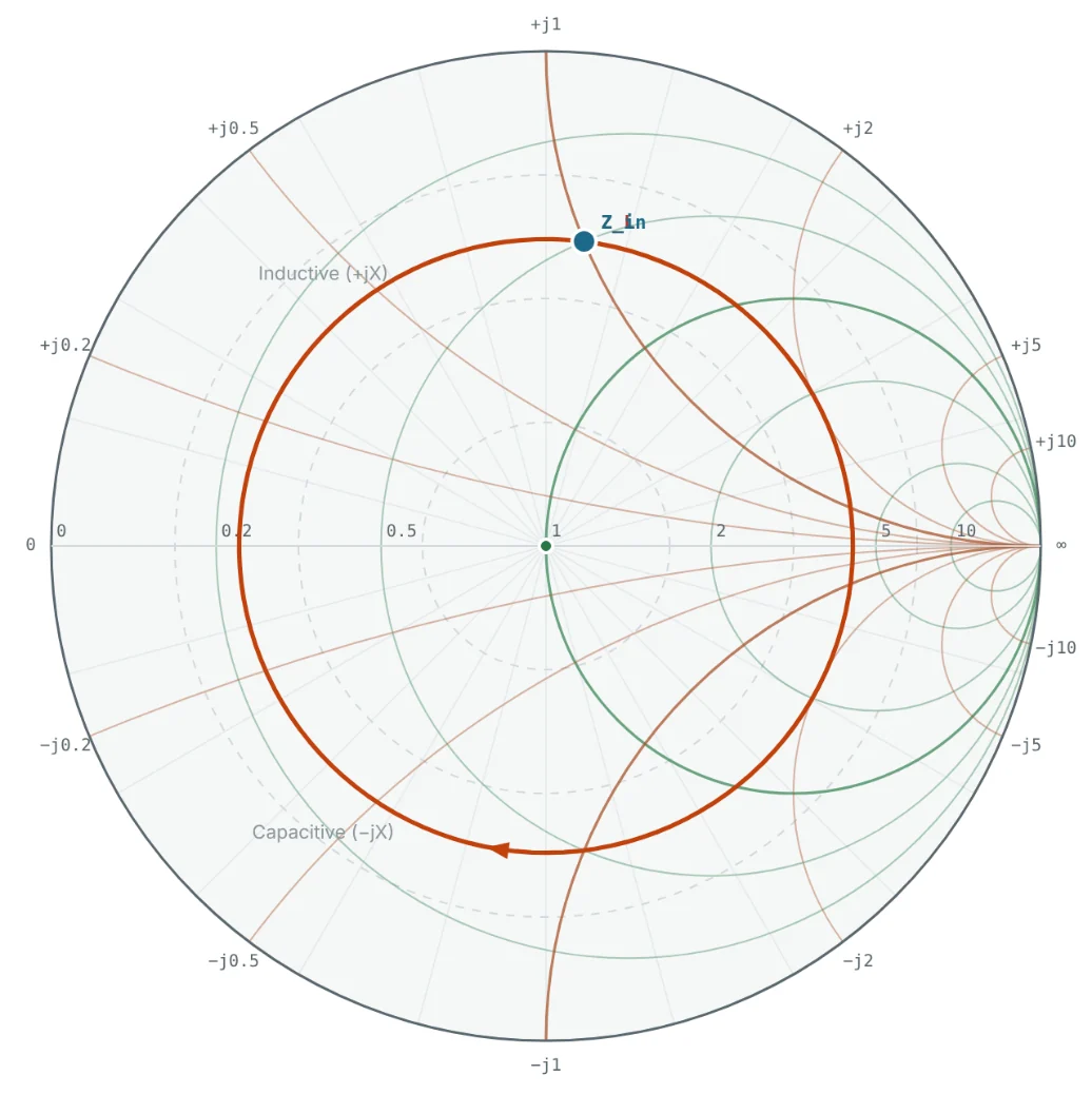
Place a compass point on the centre of the chart and draw a circle through the load point. This is the load's constant-VSWR circle (also called the constant-|Γ| circle). Every impedance seen looking toward the load along a lossless line lies on this circle, because the line changes only the angle of Γ, not its magnitude.

Moving toward the generator (away from the load) rotates the point clockwise.
Moving toward the load rotates it anticlockwise.
One full turn is λ/2 of line, because Γ rotates by 2βd = 720° per wavelength.

That is how Fig 1 was produced: adding a 0.5λ line in the calculator rotates the point once around its VSWR circle and back to where it started.

Finding the Reflection Coefficient

Magnitude. |Γ| is the distance from the centre to the point, as a fraction of the chart radius. On paper, measure both with a ruler and divide, or transfer the distance to the "reflection coefficient" scale printed below most charts.

Angle. Draw a line from the centre through the point to the rim and read the angle on the outer "angle of reflection coefficient" scale. 0° points to the right (open-circuit end), +90° to the top, ±180° to the left (short-circuit end) and −90° to the bottom.

Calculator readouts for 25 + j50 ohms: input impedance, reflection coefficient 0.620 at 82.9 degrees, S11 minus 4.15 dB and VSWR 4.27 — Fig 4 — The calculator reads the same values numerically: Γ = 0.620 ∠ 82.9°, S11 = −4.15 dB, VSWR = 4.27 : 1 and Y = 8 − j16 mS. Try it in the Smith Chart Calculator →

Determining VSWR From the Chart

The VSWR circle crosses the horizontal axis at two points. Where it crosses the right-hand axis (r > 1), the normalised resistance equals the VSWR directly. Where it crosses the left-hand axis, the resistance is 1/VSWR. No calculation is needed — read the r label at the crossing.

Fig 5 — The VSWR circle of z = 0.5 + j1 crosses the right axis at r = 4.27 (= VSWR, a voltage maximum) and the left axis at r = 0.234 (= 1/VSWR, a voltage minimum)

VSWR circle, |Γ| = 0.62

VSWR, return loss and mismatch loss from |Γ|

VSWR = \frac{1 + | Γ |}{1 - | Γ |} RL = - 20 \log_{10} | Γ | ML = - 10 \log_{10} (1 - {| Γ |}^{2})

The relationships behind VSWR and return loss are developed in Part 4. Paper charts print VSWR, return-loss and |Γ| scales below the chart so all three can be read with a pair of dividers.

Converting Plotted Values Back to Actual Impedance

Any point read off the chart is normalised. Multiply by Z₀ to get ohms. For admittance, use the fact that rotating a point by 180° about the centre turns z into its reciprocal y = 1/z — the point diametrically opposite on the VSWR circle. Then divide by Z₀ (or multiply by Y₀ = 1/Z₀) to get siemens:

Denormalising impedance and admittance

Z = z \cdot Z_{0} y = \frac{1}{z} (180° rotation) Y = \frac{y}{Z_{0}}

Fig 6 — z = 0.5 + j1 and its admittance y = 0.4 − j0.8 lie at opposite ends of a diameter of the VSWR circle

VSWR circle

Step-by-Step Solved Examples

All examples use Z₀ = 50 Ω. Each load can be entered directly in the Smith Chart Calculator to check the graphical result.

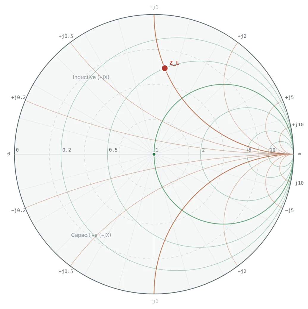
Inductive Load: 25 + j50 Ω

Problem: Plot Z_L = 25 + j50 Ω and find Γ, VSWR, return loss and the load admittance.

Normalise: z = (25 + j50)/50 = 0.5 + j1.
Plot: intersection of the r = 0.5 circle and the x = +1 arc (Fig 2) — upper half, inductive.
VSWR circle: centred on the chart through the point; it crosses the right axis at r ≈ 4.27.
Γ: the point is 0.62 of the radius from the centre at 82.9° → Γ = 0.620 ∠ 82.9°.
Return loss: −20 log 0.620 = 4.15 dB.
Admittance: rotate 180° → y = 0.4 − j0.8 → Y = (0.4 − j0.8)/50 = 8 − j16 mS.

Answer: Γ = 0.620 ∠ 82.9°, VSWR = 4.27, RL = 4.15 dB, Y = 8 − j16 mS

All four values match the calculator readout in Fig 4 exactly. With a VSWR above 4, about 38% of the incident power is reflected — this load needs matching (we match it in Part 10).

Capacitive Load: 75 − j25 Ω

Problem: Plot Z_L = 75 − j25 Ω and find Γ, VSWR and return loss. Does it meet a −10 dB S11 specification?

z = 1.5 − j0.5

Γ = \frac{0.5 - j 0.5}{2.5 - j 0.5} = 0.231 - j 0.154 = 0.277 ∠ - 33.7 ° VSWR = 1.77 RL = 11.1 dB

Smith chart with the load 75 minus j25 ohms plotted inside the r = 1 circle in the lower capacitive half — The point is in the lower (capacitive) half, inside the r = 1 circle because r = 1.5 > 1, and close to the centre. Try it in the Smith Chart Calculator →

Calculator readouts for 75 minus j25 ohms: Γ 0.277 at minus 33.7 degrees, S11 minus 11.14 dB, VSWR 1.77 — Calculator readout: S11 = −11.14 dB, better than the −10 dB target. Try it in the Smith Chart Calculator →

Answer: Γ = 0.277 ∠ −33.7°, VSWR = 1.77, RL = 11.1 dB — passes a −10 dB specification

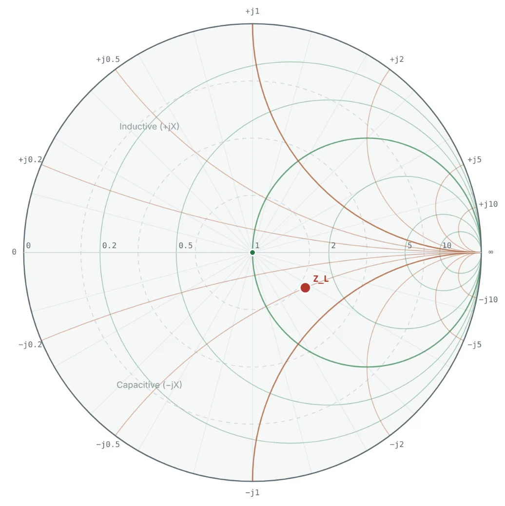
The −10 dB contour is the circle |Γ| = 0.316 (VSWR 1.92). Any load plotted inside that circle meets the spec, which is why VSWR circles are such a fast visual check.

Low-Resistance Load: 10 Ω

Problem: A power transistor presents 10 Ω (resistive) to a 50 Ω line. Plot it and read the VSWR without using the formula.

Smith chart with a 10 ohm load on the left part of the horizontal axis — z = 0.2 lies on the horizontal axis, far to the left — between the centre and the short-circuit end. Try it in the Smith Chart Calculator →

Calculator readouts for 10 ohms: Γ 0.667 at 180 degrees, S11 minus 3.52 dB, VSWR 5.00 — Calculator readout: Γ = 0.667 ∠ 180°, VSWR 5.00 : 1. Try it in the Smith Chart Calculator →

Answer: z = 0.2, Γ = 0.667 ∠ 180°, VSWR = 5.0

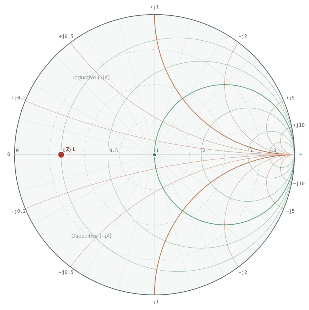
The VSWR circle through z = 0.2 crosses the right axis at r = 1/0.2 = 5, so the VSWR is 5 by inspection. Low-impedance loads like this are typical of power amplifier outputs and are matched with low-pass L or π networks.

Reading an Impedance Back From the Chart

Problem: A VNA marker shows a point at |Γ| = 0.45, angle 120°. What are the impedance and the VSWR?

Γ = 0.45∠120° = −0.225 + j0.390; z = (1 + Γ)/(1 − Γ)

z = \frac{0.775 + j 0.390}{1.225 - j 0.390} = 0.483 + j 0.472 Z = 24.1 + j 23.6 Ω VSWR = \frac{1.45}{0.55} = 2.64

Answer: Z ≈ 24.1 + j23.6 Ω, VSWR ≈ 2.64

On the chart the point sits just outside the r = 0.5 circle and just below the x = +0.5 arc — reading r ≈ 0.48 and x ≈ 0.47 by eye gives the same answer to two figures, which is the usual accuracy of a paper chart.

Voltage Maximum and Minimum Positions

Problem: For the 25 + j50 Ω load, how far from the load is the first voltage maximum on the line, and what impedances are seen at the voltage maximum and minimum?

Rotate clockwise from ∠Γ = 82.9° to 0° (right axis); 360° of chart rotation = 0.5λ

d_{max} = \frac{82.9 °}{720 °} λ = 0.115 λ Z_{max} = 4.27 \times 50 = 213 Ω Z_{min} = \frac{50}{4.27} = 11.7 Ω

Answer: first V_max at 0.115λ from the load (Z = 213 Ω); V_min a further 0.25λ on, at 0.365λ (Z = 11.7 Ω)

The green arrow in Fig 5 shows this rotation. At 2.4 GHz on air-dielectric line (λ = 125 mm) the maximum is 14.4 mm from the load. Measuring the position of a voltage minimum on a slotted line was, for decades, how unknown loads were found — the Smith chart turned that measurement back into an impedance.

Summary

Step	Action	Result for 25 + j50 Ω
1. Normalise	z = Z_L / Z₀	0.5 + j1
2. Plot	Intersect r circle and x arc	Upper half, outside r = 1 circle
3. VSWR circle	Centre → through point	\|Γ\| = 0.62
4. Γ	Radius ratio and rim angle	0.620 ∠ 82.9°
5. VSWR	r at right-axis crossing	4.27
6. Return loss	−20 log\|Γ\|	4.15 dB
7. Admittance	Rotate 180°, divide by Z₀	8 − j16 mS
8. Line effect	Rotate clockwise toward generator	V_max at 0.115λ

Always normalise first; the same load is a different point in a 50 Ω and a 75 Ω system.
The impedance point is the unique intersection of one r circle and one x arc.
The circle centred on the chart through the point is the constant-VSWR circle; a lossless line moves the point around it.
The VSWR is the r value where that circle crosses the right-hand axis; the admittance is the diametrically opposite point.

With plotting mastered, Part 10: Impedance Matching Using the Smith Chart uses these moves to bring a load to the centre of the chart — designing real matching networks.

Put It Into Practice

Use the NEXT ANTENNAS calculators to apply the ideas from this article to real designs.

Antenna Design Patch Antenna Calculator Width, length, effective permittivity and inset feed of a rectangular microstrip patch for your frequency and substrate. Open calculator → Transmission Lines Microstrip Calculator Trace width for a target impedance, effective permittivity and guided wavelength on any PCB substrate. Open calculator → Impedance Matching Smith Chart Visualiser Plot impedances, reflection coefficient and VSWR, and build matching networks step by step. Open calculator → All Tools All RF Calculators Browse every NEXT ANTENNAS calculator for RF, microwave and antenna design in one place. Open calculator →