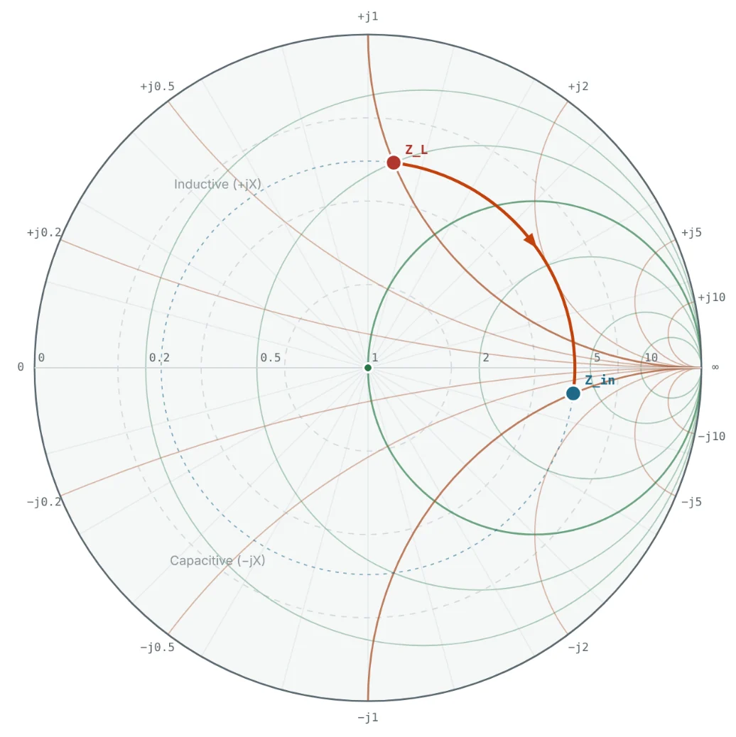
Why the Line Changes the Impedance
In Part 4 we saw that the voltage and current along a mismatched line vary from point to point. Their ratio — the impedance you would measure if you cut the line there and looked toward the load — varies too. A length of line placed in front of a load therefore acts as an impedance transformer. Sometimes that is a nuisance (a cable makes an antenna look different from what it is); sometimes it is a tool (a quarter-wave section matches two different impedances).
The full derivation of the input impedance equation, lossy lines and the propagation constant γ = α + jβ are covered in our transmission line series. Here we focus on using the result and seeing it on the Smith chart. Open the Transmission Line Theory series →
The Input Impedance Equation
The same result is simpler in terms of the reflection coefficient. Moving a distance ℓ toward the source delays the reflected wave by 2βℓ relative to the forward wave:
Transformation as Rotation on the Smith Chart
Since Γ_in has the same magnitude as Γ_L and an angle reduced by 720° × ℓ/λ, adding line in front of a load moves the impedance point clockwise around the chart's centre on its VSWR circle. Moving toward the load moves it counter-clockwise.
| Line length ℓ | Electrical length βℓ | Rotation on the chart | Effect on Z_L |
|---|---|---|---|
| λ/8 | 45° | 90° clockwise | Quarter of a turn: resistive loads become complex, z = 1 + jx loads lie on a circle |
| λ/4 | 90° | 180° | Inverts the normalised impedance: z_in = 1/z_L |
| λ/2 | 180° | 360° (full turn) | Repeats the load: Z_in = Z_L |
Printed Smith charts carry an outer scale marked "wavelengths toward generator" (WTG) running clockwise from 0 to 0.5. Because half a wavelength is one full turn, the scale only needs to cover 0.5 λ. To find the impedance through a line of length ℓ, read the load's WTG position, add ℓ/λ and draw a line from the centre to the new position. Part 8 explains these scales in detail.
The Quarter-Wave Transformer
At ℓ = λ/4, tan βℓ → ∞ and the input impedance equation reduces to a remarkably simple result:
On a Smith chart normalised to the system Z₀, a quarter-wave section of a different impedance Z₁ does not rotate around the chart's centre, but around the point z = Z₁/Z₀ on the real axis. The calculator draws exactly that arc:
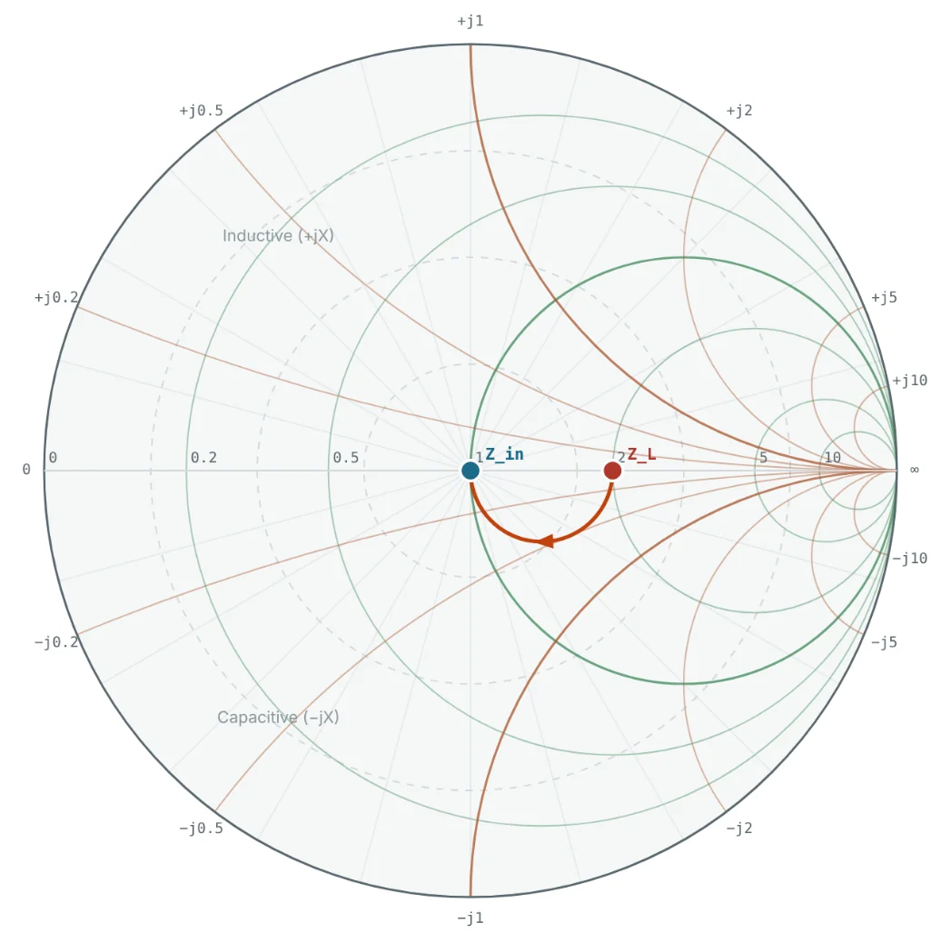

The quarter-wave transformer is narrow-band — it is exactly λ/4 at only one frequency — and only matches real impedances. A complex load must first be rotated onto the real axis by a length of Z₀ line (Example 5 of Part 4 found that distance: 0.115 λ for 25 + j50 Ω). Multi-section transformers widen the bandwidth.
The Half-Wavelength Line
At ℓ = λ/2, tan βℓ = 0 and Z_in = Z_L regardless of Z₀. A half-wave line is "invisible" at its design frequency, which is useful for placing a load at a distance without changing its impedance — for example, connecting an antenna through a cable cut to a multiple of λ/2. The full-circle screenshot in Part 4 shows exactly this: 25 + j50 Ω comes back to itself after λ/2.
Short- and Open-Circuited Stubs
Setting Z_L = 0 or ∞ in the input impedance equation gives a pure reactance whose value depends on the length:
Stubs are how distributed circuits make inductors and capacitors without lumped parts. Part 11 builds complete matching networks from them.
From Electrical to Physical Length
The fractions of λ above are wavelengths on the line, which are shorter than in free space by the velocity factor VF = 1/√ε_eff:
| Medium at 2.4 GHz | VF | λ | λ/4 | λ/8 |
|---|---|---|---|---|
| Air line | 1.00 | 124.9 mm | 31.2 mm | 15.6 mm |
| Solid-PE coax (RG-58, RG-213) | 0.66 | 82.4 mm | 20.6 mm | 10.3 mm |
| 50 Ω microstrip, 1.6 mm FR-4 (ε_eff ≈ 3.32) | 0.55 | 68.6 mm | 17.1 mm | 8.6 mm |
Worked Examples
25 + j50 Ω Through λ/8 of 50 Ω Line
Problem: Find the input impedance of a λ/8 length of 50 Ω line terminated in 25 + j50 Ω.

The inductive load now looks capacitive and four times larger in resistance — same |Γ|, angle reduced by 90°.
Designing a Quarter-Wave Transformer
Problem: Match a 100 Ω resistive load to a 50 Ω system at 2.4 GHz with a quarter-wave microstrip section on 1.6 mm FR-4.
The calculator confirms Z_in = 50 + j0 Ω. On FR-4 the 70.7 Ω trace is narrower than a 50 Ω trace (about 1.6 mm instead of 3.1 mm) and has a slightly lower ε_eff (≈ 3.17), so its λ/4 is about 17.5 mm rather than 17.1 mm — use the Microstrip Calculator for both numbers.
Impedance Inversion by a Quarter Wave
Problem: What does 25 + j50 Ω look like through λ/4 of 50 Ω line?
The point is diametrically opposite the load on the chart (Fig 2). Since 1/z is the normalised admittance, a λ/4 line also explains why rotating 180° turns the Smith chart into an admittance chart (Part 6).
A Short-Circuit Stub as an Inductor
Problem: A λ/8 short-circuited 50 Ω stub is used at 2.4 GHz. What inductance does it replace?
Unlike a real inductor, the stub's reactance follows tan βℓ, not ωL, so the equivalence holds only near 2.4 GHz.
Physical Quarter-Wave Lengths
Problem: How long is λ/4 at 2.4 GHz in air, in VF 0.66 coax, and as 50 Ω microstrip on FR-4 (ε_eff = 3.32)?
Always convert using the velocity factor of the actual line — cutting a coax "quarter wave" to the free-space length is a classic mistake.
Summary
- Z_in = Z₀(Z_L + jZ₀ tan βℓ)/(Z₀ + jZ_L tan βℓ); equivalently Γ_in = Γ_L e^(−j2βℓ).
- A lossless line rotates the impedance clockwise on its VSWR circle by 720° × ℓ/λ; λ/2 is one full turn.
- λ/4 inverts the normalised impedance; a λ/4 section of Z₁ = √(Z_in Z_L) matches two real impedances.
- Short and open stubs produce pure reactances and act as distributed inductors and capacitors.
- Convert electrical length to physical length with the line's velocity factor.
We now have every ingredient — impedance, Z₀, Γ, VSWR and rotation along a line. Part 6: Introduction to the Smith Chart brings them together in one graphical tool.
Put It Into Practice
Use the NEXT ANTENNAS calculators to apply the ideas from this article to real designs.