Reading the Chart as Families of Circles
In Part 6 we built the Smith chart by mapping the right half of the impedance plane into the Γ unit disc, and in Part 7 we normalised impedances to plot them. The mapping Γ = (z − 1)/(z + 1) has a special property: it turns straight lines into circles. Every line of constant r or constant x in the impedance plane becomes a circle (or an arc of one) in the Γ plane. Knowing where each family's circles sit — and why — makes the chart quick and reliable to read.
Constant-Resistance Circles
Constant-resistance circles: all touch at the right edge.
Constant-reactance arcs: inductive above, capacitive below.
Constant-Reactance Arcs
Every r circle crosses every x arc at a right angle, which is why the grid looks "curvilinear-square" and why reading a point is unambiguous: one circle, one arc, one intersection.
Constant-Conductance and Susceptance Circles
The admittance grid is the impedance grid rotated by 180° (because y = 1/z corresponds to Γ → −Γ). The equations are the same with r → g, x → b and the sign of Γ reversed:
| Family | Centre | Radius | Common point | Notes |
|---|---|---|---|---|
| Constant r | (r/(1+r), 0) | 1/(1+r) | Open (+1) | r = 1 through the centre |
| Constant x | (1, 1/x) | 1/|x| | Open (+1) | +x above the axis |
| Constant g | (−g/(1+g), 0) | 1/(1+g) | Short (−1) | g = 1: centre (−0.5, 0), radius 0.5 |
| Constant b | (−1, −1/b) | 1/|b| | Short (−1) | +b (capacitive) below the axis |
| Constant |Γ| (VSWR) | (0, 0) | |Γ| | — | Crosses real axis at r = VSWR and 1/VSWR |
| Constant Q | (0, ∓1/Q) | √(1 + 1/Q²) | Short and open | Upper and lower arcs |
A capacitor adds positive susceptance (+jb) but negative reactance (−jx). On a combined Z/Y chart both describe the same physical point, so capacitive loads — and +b arcs — are in the lower half. Mixing up the sign of b is the most common mistake in shunt-element matching.
The g = 1 circle deserves special attention: it is the impedance r = 1 circle reflected through the centre, and it is where every shunt-element match must arrive before the final shunt component cancels the susceptance. Part 10 uses it repeatedly.
Constant-VSWR Circles
Circles centred on the chart centre have constant |Γ| and therefore constant VSWR and return loss. As shown in Part 5, a lossless line moves an impedance around its VSWR circle. The circle crosses the right half of the real axis at r = VSWR, so the r value of that crossing is the VSWR — no calculation needed. The −10 dB return-loss circle (|Γ| = 0.316, VSWR 1.92) is a useful target to keep in mind: any point inside it meets the common S11 < −10 dB specification.
The Outer Scales
Printed Smith charts carry three rings of scales around the edge:
- Wavelengths toward generator (WTG) — runs clockwise from 0 at the short-circuit point to 0.5 λ back at the same point. Moving toward the source along the line means increasing WTG.
- Wavelengths toward load (WTL) — the same scale running counter-clockwise.
- Angle of reflection coefficient — from 0° at the right (open) through ±90° at the top and bottom to ±180° at the left (short).
Below the chart, most printed versions also carry radially scaled parameters: rulers that convert the distance from the centre (|Γ|) into VSWR, return loss, mismatch loss, power reflection coefficient and dBS (standing wave ratio in dB). Set a pair of dividers from the centre to the point, transfer it to the ruler, and read all of them at once. Digital tools such as the Smith Chart Calculator display these values directly.
Constant-Q Curves
For any impedance, the node quality factor Q_n = |x|/r = |X|/R. All points with the same Q_n lie on an arc that runs from the short-circuit point to the open-circuit point:
Constant-Q curves are a design tool: the loaded Q of a two-element L-network is approximately the highest Q_n its path touches, and its fractional bandwidth is roughly 1/Q. Keeping a matching path inside a low-Q arc gives a wider-band match. The calculator can overlay Q curves:
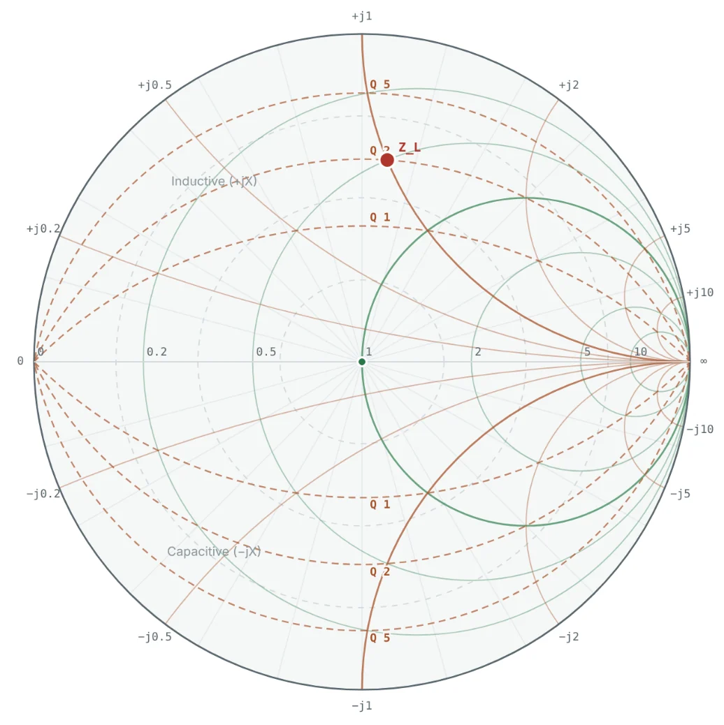
The same curves from the equation above.
Worked Examples
Reading Every Parameter of 50 + j50 Ω
Problem: For Z = 50 + j50 Ω on a 50 Ω chart, find which r circle and x arc it lies on, Γ, VSWR and the admittance.
Being on the r = 1 circle means a single series reactance of −j1 (a capacitor of −j50 Ω) would match it — the idea behind Part 10.
Using the Wavelength Scale
Problem: Find the WTG position of z = 1 + j1 and the impedance after 0.1 λ of 50 Ω line.
The point has just crossed the open-circuit side of the real axis (0.25 λ), so it changed from inductive to slightly capacitive.
Locating the g = 1 Circle
Problem: Find the centre and radius of the g = 1 circle, and verify that y = 1 + j1 lies on it.
y = 1 + j1 is in the lower half (capacitive), as expected for positive susceptance.
Node Q and Expected Bandwidth
Problem: Find Q_n for 25 + j50 Ω and estimate the fractional bandwidth of a narrow-band match through this point.
This is only an estimate — the actual −10 dB bandwidth depends on the matching path. In Part 10, the four L-networks for this load give −10 dB bandwidths ranging from about 37% to over 100%, depending on which side of the chart the path takes.
Summary
- Constant-r circles and constant-x arcs all meet at the open-circuit point; constant-g circles and constant-b arcs meet at the short-circuit point.
- The admittance grid is the impedance grid rotated 180°; positive susceptance lies in the lower half.
- Constant-VSWR circles are centred on the chart; a lossless line moves along them, and r at the right-hand crossing equals the VSWR.
- The WTG scale converts line length to rotation: 0.5 λ is a full turn.
- Constant-Q arcs indicate how narrow-band a matching path will be.
With every circle understood, Part 9: How to Plot Impedance on a Smith Chart puts them to work, step by step.
Put It Into Practice
Use the NEXT ANTENNAS calculators to apply the ideas from this article to real designs.