Why Match Impedances?
Through Parts 3 to 9 we have measured mismatch in many ways — Γ, return loss, VSWR — and learned to read it on the Smith chart. Now we remove it. A matching network is a lossless (or nearly lossless) circuit inserted between the line and the load that transforms the load into Z₀ at the design frequency. With a perfect match:
- no power is reflected, so all available power reaches the load;
- the line carries only a forward wave (VSWR 1 : 1), so voltage peaks and cable stress are minimised;
- the source sees its design load, so amplifiers deliver their rated power, gain and stability;
- in receivers, the noise and gain performance of the front end depend on the impedance it sees.
Maximum Power Transfer and Conjugate Matching
A source with internal impedance Z_S delivers the most power to a load when the load is the complex conjugate of the source:
In most RF work both the source and the line are 50 Ω, so "matching" means moving the load to the chart centre. The same techniques apply to conjugate matching between two complex impedances: the target point is then Z_S* instead of the centre.
How Components Move the Impedance
A series component adds reactance without changing resistance, so the point slides along its constant-r circle. A shunt component adds susceptance without changing conductance, so the point slides along its constant-g circle. The direction depends on the component type:
| Component | Adds | Moves along | Direction on the chart |
|---|---|---|---|
| Series inductor | +jX (= jωL) | constant-r circle | Clockwise (upward) |
| Series capacitor | −jX (= −j/ωC) | constant-r circle | Counter-clockwise (downward) |
| Shunt capacitor | +jB (= jωC) | constant-g circle | Clockwise (downward) |
| Shunt inductor | −jB (= −j/ωL) | constant-g circle | Counter-clockwise (upward) |
| Series line (Z₀) | electrical length | constant-VSWR circle | Clockwise around the centre |
Inductors move the point up (toward the inductive half) on their own circle; capacitors move it down. That works for both series and shunt elements, because a shunt capacitor adds positive susceptance, which lies in the lower half of the chart.
Designing an L-Network Step by Step
An L-network uses one series and one shunt element. The idea is to use the first element to land on a circle that passes through the centre, then use the second element to slide along that circle to the centre. Two such circles exist:
- the g = 1 circle — if the element nearest the source is in shunt, the point must arrive on g = 1 before it, because a shunt element can then cancel the remaining susceptance;
- the r = 1 circle — if the element nearest the source is in series, the point must arrive on r = 1 before it.
- Normalise the load and plot z_L (and y_L).
- Choose the topology: series-at-load (aim for g = 1) or shunt-at-load (aim for r = 1).
- Move along the load's own r circle (series element) or g circle (shunt element) until you hit the target circle. Usually there are two intersections.
- Read the change in x or b — that is the first element.
- From the intersection, the second element cancels the remaining reactance or susceptance to reach the centre.
- Denormalise and convert to L and C values (Part 7).
If the load lies inside the r = 1 circle (R_L > Z₀), a series element at the load can never reach the g = 1 circle — you must start with a shunt element. If the load lies inside the g = 1 circle (G_L > Y₀), you must start with a series element. Our example load, z = 0.5 + j1 (g = 0.4), is outside both circles, so all four L-network solutions exist.
Matching 25 + j50 Ω at 2.4 GHz
We now match the load used throughout the series — 25 + j50 Ω (z = 0.5 + j1, y = 0.4 − j0.8) — to 50 Ω at 2.4 GHz.
Network A: Series C at the Load, Shunt C at the Source
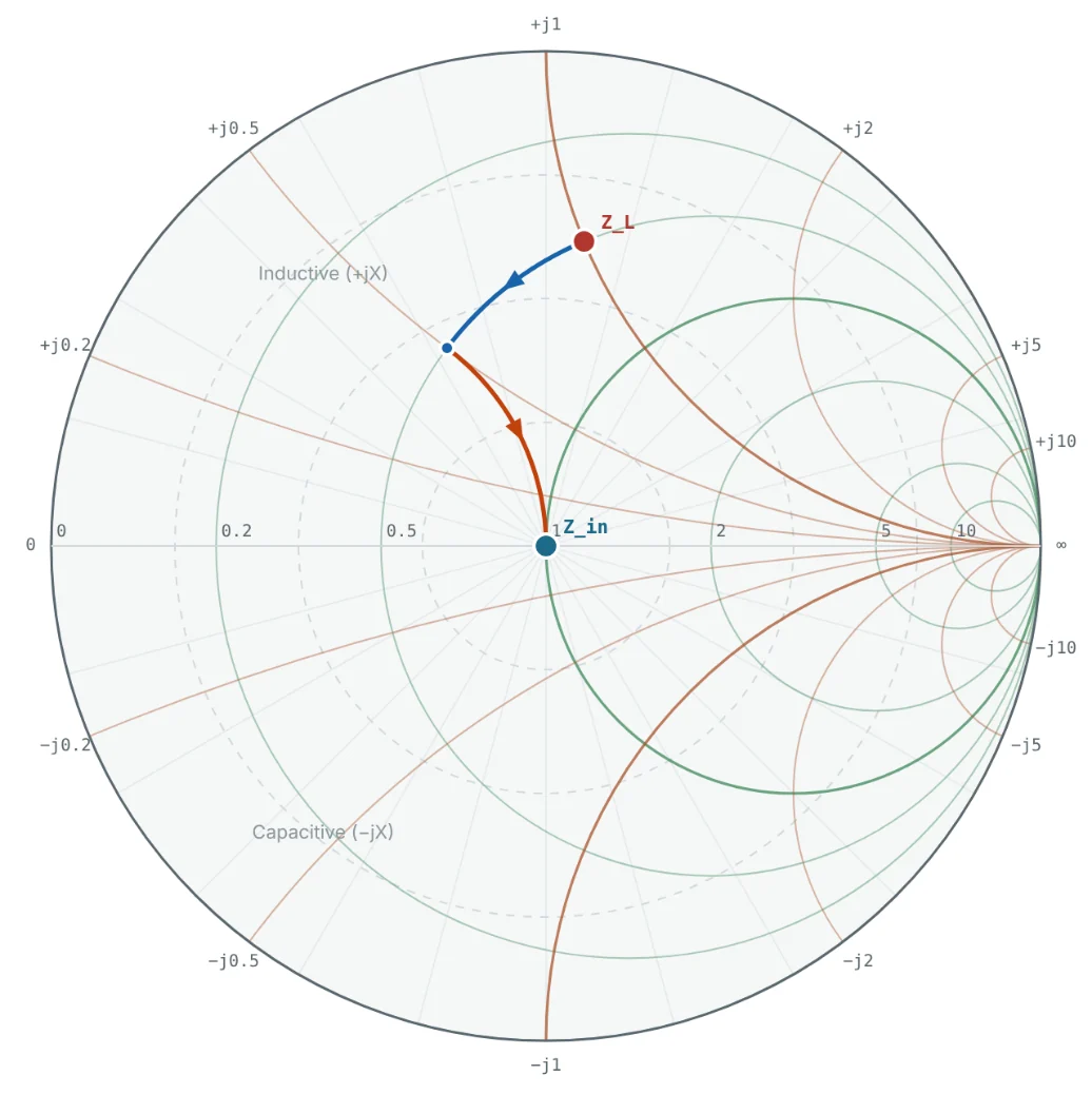
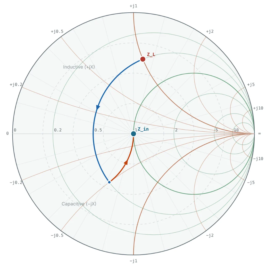
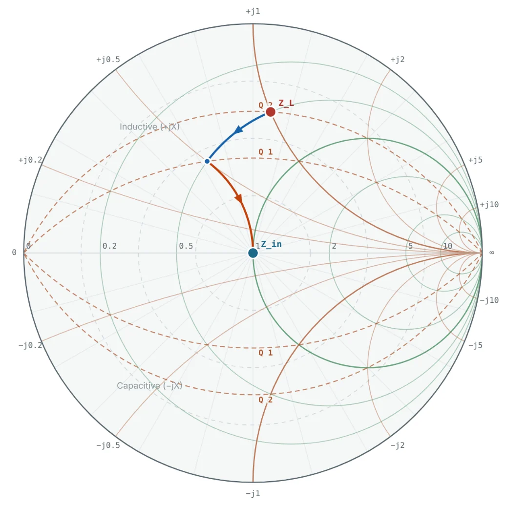
The r = 0.5 circle meets the g = 1 circle at z = 0.5 ± j0.5. Moving down from 0.5 + j1 to 0.5 + j0.5 needs Δx = −0.5: a series capacitor. At that point y = 1 − j1, so a shunt capacitor with b = +1 reaches the centre.

Network B: Series C at the Load, Shunt L at the Source
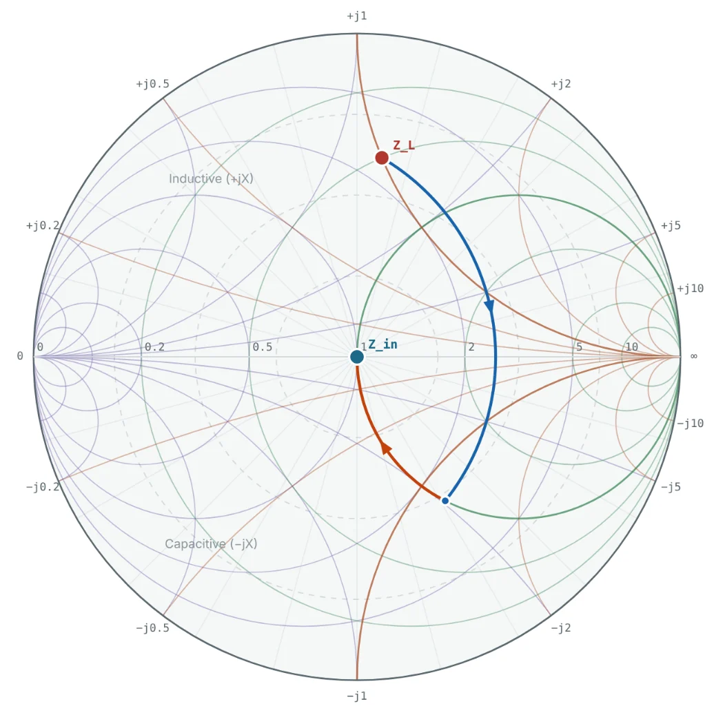
The other intersection, z = 0.5 − j0.5, needs a larger series capacitor reactance (Δx = −1.5, X = −75 Ω). There y = 1 + j1, so the shunt element must add b = −1: an inductor.
Network B: high-pass topology.
Networks C and D: Shunt Element at the Load
Starting with a shunt element, we follow the load's g = 0.4 circle until it meets r = 1. The intersections are y = 0.4 ± j0.49. From y_L = 0.4 − j0.8, both require a shunt capacitor: b = +1.29 (B = +25.8 mS) or b = +0.31 (B = +6.2 mS). They land at z = 1 − j1.22 and z = 1 + j1.22, finished by a series inductor (+61.2 Ω) or a series capacitor (−61.2 Ω).
Network C: low-pass topology.
| Network | At the load | At the source side | Intermediate point | Type |
|---|---|---|---|---|
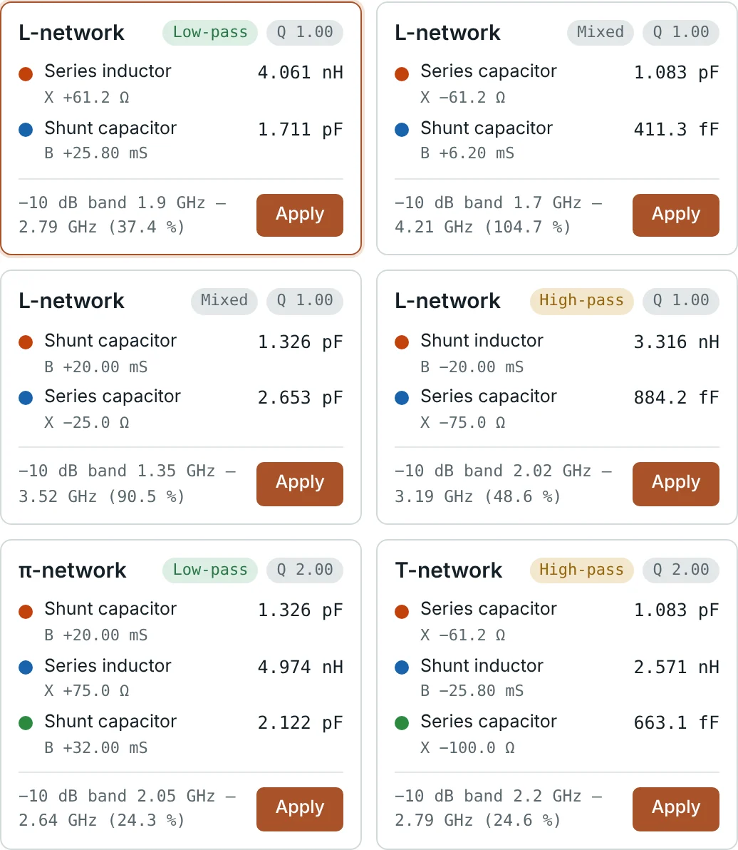
| A | Series C 2.653 pF (X = −25 Ω) | Shunt C 1.326 pF (B = +20 mS) | z = 0.5 + j0.5 | Mixed |
| B | Series C 0.884 pF (X = −75 Ω) | Shunt L 3.316 nH (B = −20 mS) | z = 0.5 − j0.5 | High-pass |
| C | Shunt C 1.711 pF (B = +25.8 mS) | Series L 4.061 nH (X = +61.2 Ω) | z = 1 − j1.22 | Low-pass |
| D | Shunt C 0.411 pF (B = +6.2 mS) | Series C 1.083 pF (X = −61.2 Ω) | z = 1 + j1.22 | Mixed |
Letting the Calculator Find Every Solution
The Smith Chart Calculator's matching solver lists all L-network solutions plus π and T networks for a chosen loaded Q, each with its −10 dB bandwidth. For 25 + j50 Ω at 2.4 GHz it returns exactly the four networks above — a useful check on a hand design.
Bandwidth and Constant-Q Curves
All four networks are perfect at 2.4 GHz, but their component reactances change with frequency differently, so their bandwidths differ greatly. The constant-Q curves of Part 8 explain why: the loaded Q of an L-network is set by the highest Q_n its path reaches, and a lower Q means a wider band. Network A's path stays between the Q = 2 and Q = 1 arcs and ends at the centre along a gentle curve.
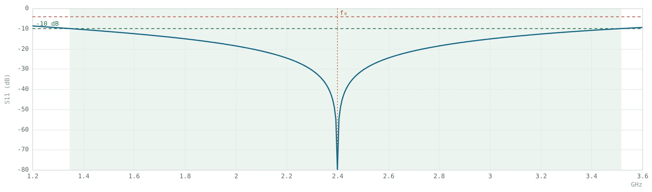

The sweep holds the load at 25 + j50 Ω at every frequency, so it measures the matching network alone. A real antenna's impedance also changes with frequency, which usually narrows the band considerably — Part 12 repeats the exercise with a measured antenna file.
To make a match narrower (for selectivity or harmonic rejection), add a third element: π and T networks let you choose a loaded Q higher than the L-network minimum. The solver's π and T networks with Q = 2 have about 24% bandwidth. To make it wider, cascade two or more L-sections, each with a small step in impedance, so that the path stays close to the real axis.
Worked Examples
Power With and Without a Conjugate Match
Problem: A source with V_S = 10 V RMS and Z_S = 25 + j50 Ω drives (a) its conjugate load 25 − j50 Ω, and (b) a plain 50 Ω load. Find the power in each.
The 2.11 dB shortfall equals the mismatch loss the calculator reports for 25 + j50 Ω on a 50 Ω system.
Component Values for Network B
Problem: Verify the values of network B: series Δx = −1.5 and shunt b = −1 at 2.4 GHz in a 50 Ω system.
A 0.884 pF capacitor is small enough that pad and package parasitics (≈ 0.1–0.2 pF) matter — one reason to prefer network A here.
Shunt-First Design: Network C
Problem: Find the shunt susceptance that takes y_L = 0.4 − j0.8 onto the r = 1 circle with a final series inductor, and the component values.

This low-pass form also attenuates harmonics, which is useful after a power amplifier.
Choosing Between the Four Networks
Problem: Which network suits (a) a transmitter that must suppress harmonics, (b) a circuit needing a DC path to ground at the input, (c) the widest possible bandwidth?
| Network | −10 dB band | Fractional BW | Property |
|---|---|---|---|
| A | 1.35–3.52 GHz | ≈ 90% | Two capacitors, blocks DC |
| B | 2.02–3.19 GHz | 48.6% | High-pass, shunt L gives DC path |
| C | 1.90–2.79 GHz | 37.4% | Low-pass, rejects harmonics |
| D | 1.70–4.21 GHz | 104.7% | Two capacitors, widest band |
Same load, same frequency, four valid answers — choosing between them is an engineering judgement the chart makes visible.
Summary
- Matching transforms the load to Z₀ (or to Z_S* for a conjugate match), maximising delivered power.
- Series elements move along constant-r circles, shunt elements along constant-g circles; inductors move up, capacitors down.
- An L-network first reaches the g = 1 or r = 1 circle, then slides to the centre; a general load has up to four solutions.
- Loads inside the r = 1 or g = 1 circle restrict which topology can be used.
- The matching path sets the bandwidth; constant-Q curves predict it, and π/T networks or multi-section designs adjust it.
Lumped components become impractical at higher frequencies. Part 11: Single-Stub and Double-Stub Impedance Matching achieves the same match with sections of transmission line alone.
Put It Into Practice
Use the NEXT ANTENNAS calculators to apply the ideas from this article to real designs.