Antenna Bandwidth and Q Factor Explained

Fig 1 — Return loss of a matched series-resonant antenna for three values of Q. The higher the Q, the narrower the band inside the −10 dB line

Q = 5 (thick dipole)Q = 10 (thin dipole)Q = 30 (patch)

Introduction to Antenna Bandwidth

IEEE 145 defines bandwidth as "the range of frequencies within which the performance of the antenna, with respect to some characteristic, conforms to a specified standard." There is no single bandwidth: an antenna has an impedance bandwidth, a gain bandwidth, a pattern bandwidth and a polarization bandwidth, and the usable bandwidth is the frequency range where all the requirements of the application are met at once.

Bandwidth is set by the antenna's stored energy. Part 3 showed that every antenna stores reactive energy in its near field, and Part 7 showed that this energy appears as reactance that changes with frequency. The quality factor Q measures that stored energy relative to the radiated power — and it turns out to determine the impedance bandwidth almost completely.

What Is Resonant Frequency?

An antenna is resonant where its input reactance is zero (Part 7). At resonance the stored electric and magnetic energies are equal and the impedance is purely resistive. Most narrowband antennas — dipoles, monopoles, patches, small loops — are used near a resonance, because the impedance there is both easy to match and slowly varying. Their bandwidth is centred on the resonant frequency f₀ and the impedance near it is well described by the series (or parallel) RLC model:

Series-resonant antenna near f₀

Z_{A} (f) = R [1 + j Q (\frac{f}{f_{0}} - \frac{f_{0}}{f})] \approx R [1 + j 2 Q δ] δ = \frac{f - f_{0}}{f_{0}}

The exact form follows from ωL − 1/ωC with Q = ω₀L/R; the approximation holds for small δ. Wideband antennas (log-periodic, spiral, horn) are not described by a single resonance; their bandwidth is set by geometry instead.

Impedance Bandwidth

The impedance bandwidth is the frequency range over which the antenna is adequately matched to its feed line — usually |S₁₁| ≤ −10 dB (VSWR ≤ 1.92), sometimes VSWR ≤ 2 (|S₁₁| ≤ −9.5 dB), and for base-station panels VSWR ≤ 1.5 (−14 dB). It is the easiest bandwidth to measure and the one most often quoted.

Understanding the −10 dB bandwidth

At −10 dB return loss, 10% of the incident power is reflected and the mismatch loss is 0.46 dB (Part 8). That is an acceptable compromise for most radios; it also means the −10 dB bandwidth is not the half-power bandwidth. A useful mental picture: inside the −10 dB band the antenna loses at most half a decibel to mismatch.

Radiation Pattern Bandwidth

The pattern bandwidth is the range over which the beam shape — beamwidth, side-lobe level, beam direction, front-to-back ratio — stays within specification. A dipole's pattern changes little until its length exceeds about 1.25 λ (Part 2), so its pattern bandwidth is far wider than its impedance bandwidth. For arrays the reverse is often true: element spacing in wavelengths changes with frequency, and grating lobes appear when d exceeds λ/(1 + |sin θ₀|) (Part 4). Frequency-scanned arrays deliberately exploit the change.

Gain Bandwidth

The gain bandwidth is the range over which the gain (or realized gain) stays within a specified amount, commonly 1 or 3 dB, of its peak. For an aperture antenna of fixed area, gain rises as f² (A_e = Gλ²/4π, Part 12), so a horn's gain bandwidth is usually defined by an allowed variation rather than a flat response. For small resonant antennas, realized gain follows the impedance match and falls off at the band edges.

Polarization Bandwidth

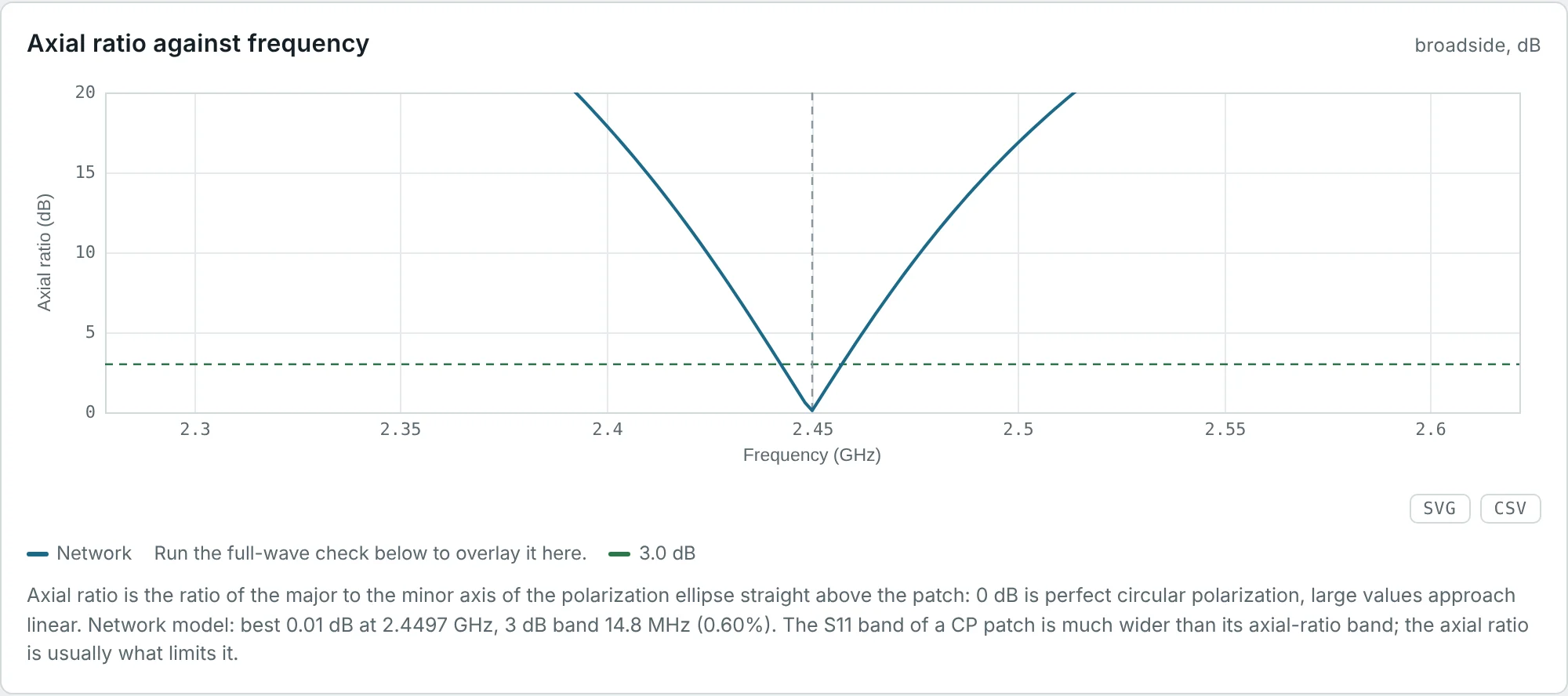
The polarization bandwidth is where the polarization remains as specified — for circularly polarized antennas, usually axial ratio ≤ 3 dB (Part 11). Single-feed CP patches produce circular polarization by exciting two orthogonal modes slightly detuned from each other; the 90° phase difference between them holds only over a narrow band. The calculator's circularly polarized patch shows how dramatic the difference can be:

Axial ratio against frequency for a corner-truncated circularly polarized patch: a sharp V shape below 3 dB only over about 15 megahertz — Axial ratio of the circularly polarized patch on RO4003C (Patch Calculator). Its −10 dB impedance bandwidth is 61.9 MHz, but the axial ratio stays below 3 dB over only 14.8 MHz (0.60%) — a quarter of it. Polarization, not impedance, limits this antenna. Try it in the Patch Antenna Calculator →

Absolute and Fractional Bandwidth

Absolute, fractional and ratio bandwidth

{BW}_{abs} = f_{H} - f_{L} FBW = \frac{f_{H} - f_{L}}{f_{c}}, f_{c} = \frac{f_{H} + f_{L}}{2} BW = f_{H} : f_{L} FBW = \frac{2 (r - 1)}{r + 1}

Narrowband antennas are described by fractional bandwidth (in %); broadband ones by the ratio r = f_H/f_L, written as "r:1". The last relation converts between the two; FBW can never exceed 200%. A common classification: narrowband below about 5%, wideband 5–25%, ultra-wideband above 25% (or above 500 MHz absolute, for the FCC UWB definition).

Antenna Quality Factor (Q)

The quality factor of an antenna is defined at resonance by the ratio of stored to dissipated energy per radian of the cycle:

Definition of antenna Q

Q = \frac{2 ω \max (W_{e}, W_{m})}{P} Q_{Z} (ω_{0}) = \frac{ω_{0}}{2 R} | Z^{'} (ω_{0}) |

P = P_rad + P_loss is the total power accepted. W_e and W_m are the stored energies, excluding the energy in the outgoing radiation itself. The second form, due to Yaghjian and Best, estimates Q directly from the measured or simulated input impedance and its frequency derivative; it reduces to (ω₀/2R)dX/dω for a series RLC (Part 7).

Antenna	Typical Q	Why
Thick dipole (L/2a ≈ 20)	4–6	Large conductor surface spreads the stored energy
Thin wire dipole (L/2a ≈ 500)	8–12	Field concentrated near the wire
Patch on a thin substrate	20–100	Energy stored in a cavity between patch and ground
Electrically small antenna (ka ≈ 0.3)	30–1000	Large reactive near field relative to radiation (Chu limit)
Small transmitting loop on HF	200–2000	Very small R_r, tiny bandwidth (a few kHz)

Relationship Between Bandwidth and Q Factor

Suppose a series-resonant antenna is matched at f₀ to a line of Z₀ = R. Using the near-resonance model above, the reflection coefficient is

Bandwidth from Q — derivation

Γ = \frac{R (1 + j 2 Q δ) - R}{R (1 + j 2 Q δ) + R} = \frac{j Q δ}{1 + j Q δ} {| Γ |}^{2} = \frac{Q^{2} δ^{2}}{1 + Q^{2} δ^{2}}

| Γ | = \frac{s - 1}{s + 1} \Rightarrow Q δ = \frac{s - 1}{2 \sqrt{s}} \Rightarrow FBW = 2 δ = \frac{s - 1}{Q \sqrt{s}}

s is the maximum allowed VSWR. The step from |Γ| to Qδ uses 1 − |Γ|² = 4s/(s + 1)². The result applies to any single-resonance antenna that is matched at its centre frequency.

Criterion	Maximum \|Γ\|	Fractional bandwidth
Half-power (3 dB mismatch)	0.707	1/Q
VSWR ≤ 2	0.333	1/(Q√2) = 0.707/Q
S₁₁ ≤ −10 dB	0.316	0.667/Q
VSWR ≤ 1.5	0.200	0.408/Q

Two consequences are worth remembering. First, loss broadens bandwidth: Q is computed with the total power P = P_rad + P_loss, so adding resistance lowers Q and widens the S₁₁ dip without improving radiation. The FR-4 patch has a wider impedance bandwidth than the Rogers patch for exactly this reason (Example 3). Second, the formula assumes a match at the centre; an antenna that is not matched to Z₀ has a different (usually smaller) bandwidth, as the 146 MHz dipole on 50 Ω shows.

The Chu Limit: How Small Can an Antenna Be?

Enclose an antenna in the smallest sphere of radius a that contains it. Chu expanded the fields outside that sphere in spherical modes and computed the minimum stored energy each mode must carry. For the lowest mode (the one radiated by a short dipole or small loop) and a lossless antenna, the minimum Q is

Chu–McLean lower bound on Q

Q_{Chu} = \frac{1}{{(k a)}^{3}} + \frac{1}{k a} Q_{lb} = e_{cd} Q_{Chu} {FBW}_{max} \approx \frac{s - 1}{Q_{lb} \sqrt{s}}

k = 2π/λ. The 1/(ka)³ term is the energy of the reactive near field outside the sphere found in Part 3. Exciting both TE and TM modes (a dipole and a loop together, as in some spherical helix designs) lowers the bound to about half. Including radiation efficiency e_cd shows how a lossy small antenna can appear to beat the limit.

Fig 2 — The Chu lower bound on Q (lossless, single mode) against electrical size ka. Q grows as 1/(ka)³ for small antennas, so halving the size multiplies the minimum Q by about eight

Q_Chu = 1/(ka)³ + 1/ka

A half-wave dipole fits in a sphere with ka = π/2, where Q_Chu ≈ 0.9; its actual Q of about 8 is far above the bound because a thin wire uses the sphere's volume poorly. Electrically small antennas (ka < 0.5) are always close to the bound in practice, and their designers trade size, bandwidth and efficiency against each other: small, wideband, efficient — pick two.

The Bode–Fano limit on matching

Can a matching network beat the single-resonance bandwidth? Partly. Bode and Fano showed that for a load consisting of a resistance R and a reactance with quality factor Q, any lossless matching network satisfies

Bode–Fano criterion and the best possible bandwidth

\int_{0}^{\infty} \ln \frac{1}{| Γ (ω) |} d ω \leq \frac{π ω_{0}}{Q} \Rightarrow {FBW}_{max} = \frac{π}{Q \ln (1 / Γ_{m})}

The second form is the limit for a rectangular |Γ| response equal to Γ_m in band and 1 outside. It is reached only with an infinite number of matching elements; a two- or three-section network reaches roughly 50–70% of it.

Factors Affecting Antenna Bandwidth

Factor	Effect
Electrical size ka	Smaller antennas have higher minimum Q (Chu limit)
Conductor thickness	Thicker dipoles (low L/2a) have flatter reactance and lower Q (Part 7, Fig 1)
Substrate thickness h	Patch bandwidth grows roughly in proportion to h/λ
Substrate permittivity ε_r	Higher ε_r stores more energy under the patch: narrower bandwidth, smaller patch
Loss	Widens the S₁₁ bandwidth by lowering Q — at the cost of efficiency
Feed and matching	A matching network can widen bandwidth up to the Bode–Fano limit
Antenna type	Travelling-wave and frequency-independent antennas avoid a single resonance altogether

For a rectangular patch, a widely used design estimate (Jackson and Alexopoulos) of the VSWR ≤ 2 bandwidth of a lossless patch is

Approximate patch bandwidth

{FBW}_{VSWR \leq 2} \approx 3.77 \frac{ε_{r} - 1}{ε_{r}^{2}} \frac{W}{L} \frac{h}{λ_{0}}

Valid for thin substrates (h ≪ λ₀). Bandwidth is linear in h and falls with ε_r. Dielectric and conductor losses add to it, which is why lossy FR-4 patches measure wider than this formula predicts.

Techniques for Bandwidth Enhancement

Technique	Principle	Typical result
Fatter conductors, bowties, biconicals	Lower stored energy per radiated power	Dipole: 10% → 30–100%
Thicker, low-ε_r substrate (or air)	Lower patch Q	Patch: 2% → 8–10%
Stacked or parasitic patches	Two coupled resonances placed side by side	15–30%
U-slot, E-shaped patch, L-probe feed	Extra resonance and compensation of the probe inductance	20–40%
Aperture-coupled feed	Tuning stub and slot resonance add a second pole	10–25%
Broadband matching networks	Multi-section networks approach the Bode–Fano limit	×1.5–3 the native bandwidth
Travelling-wave antennas	No standing wave; current decays along the structure (rhombic, Vivaldi, helix in axial mode)	2:1 to 10:1
Frequency-independent geometry	Shape defined only by angles (spiral) or self-scaling (log-periodic)	10:1 to 40:1
Self-complementary structures	Metal and slot have the same shape: Z = η/2 = 188.5 Ω at all frequencies (Mushiake)	Theoretically unlimited

Worked Examples

Fractional and Ratio Bandwidth

Problem: Express the 2.4 GHz Wi-Fi band (2400–2483.5 MHz) as a fractional bandwidth and the UWB band (3.1–10.6 GHz) as a ratio and as a fractional bandwidth.

{FBW}_{Wi-Fi} = \frac{83.5}{2441.75} = 3.42 % r = \frac{10.6}{3.1} = 3.42 : 1 {FBW}_{UWB} = \frac{2 (3.42 - 1)}{3.42 + 1} = 109 %

Answer: Wi-Fi 3.42%; UWB 3.42:1 or 109%

A Wi-Fi antenna is a narrowband design problem (one resonance with Q below about 20 will do); a UWB antenna needs a non-resonant geometry such as a planar monopole disc or a Vivaldi.

Dipole Bandwidth from Its Q

Problem: Part 7 estimated Q ≈ 8 for the 146 MHz wire dipole. Predict its VSWR ≤ 2 bandwidth if it were matched to its own resistance at resonance.

FBW = \frac{1}{8 \sqrt{2}} = 8.8 % = 12.9 MHz

Answer: about 8.8% (12.9 MHz)

Fed directly with 50 Ω, the calculator gives 9.64 MHz (6.6%): the 72 Ω / 50 Ω mismatch at the centre uses up part of the allowed VSWR. A 60 Ω quarter-wave transformer (Part 8) would recover most of the difference over the central part of the band.

Patch Bandwidth from Q: FR-4 vs Rogers

Problem: The calculator reports Q = 27.6 for the FR-4 patch and Q = 44.4 for the Rogers patch, both matched at 2.45 GHz. Predict the −10 dB bandwidths and compare with the calculated 60.7 MHz and 33.9 MHz.

{BW}_{FR4} = \frac{0.667}{27.6} \times 2450 = 59.2 MHz {BW}_{RO} = \frac{0.667}{44.4} \times 2450 = 36.8 MHz

Answer: 59 MHz and 37 MHz, within 3% and 9% of the calculator's full results

The FR-4 patch is "wider" only because half of its power is burned in the substrate (Part 9). Its realized gain is 3 dB lower across the whole band.

Chu Limit for a 2.45 GHz Module Antenna

Problem: A Bluetooth antenna must fit in a sphere of radius 1 cm. Find the minimum Q and the maximum VSWR ≤ 2 bandwidth for a lossless single-mode antenna.

k a = \frac{2 π \times 0.01}{0.1224} = 0.513 Q_{Chu} = \frac{1}{{0.513}^{3}} + \frac{1}{0.513} = 7.39 + 1.95 = 9.3 FBW \leq \frac{1}{9.3 \sqrt{2}} = 7.6 %

Answer: Q ≥ 9.3; bandwidth at most 7.6% (186 MHz)

The 83.5 MHz ISM band needs 3.4%, so a 2 cm antenna can cover it with margin — consistent with the chip and PCB antennas in every Bluetooth product.

Covering LTE Band 8 with a Tiny Antenna

Problem: An IoT antenna for 880–960 MHz must fit in a sphere of radius 2 cm. Can a lossless antenna cover the band with VSWR ≤ 2? What if the efficiency is 40%?

k a = 0.377 Q_{Chu} = 21.3 \Rightarrow FBW \leq 3.3 % Q_{lb} = 0.4 \times 21.3 = 8.5 \Rightarrow FBW \leq 8.3 %

Answer: no — the band needs 8.7% and a lossless antenna allows 3.3%; at 40% efficiency the bound rises to 8.3%, almost enough

This is why small cellular antennas are either tunable (switching between sub-bands) or accept low efficiency. A matching network can add up to the Bode–Fano gain (Example 6).

What a Matching Network Can Add

Problem: An antenna has Q = 10. Compare its single-resonance −10 dB bandwidth with the Bode–Fano limit for |Γ| ≤ 0.316.

{FBW}_{single} = \frac{0.667}{10} = 6.7 % {FBW}_{BF} = \frac{π}{10 \ln (1 / 0.316)} = 27 %

Answer: 6.7% without matching, at most 27% with an ideal network — a factor of 4

A practical double-tuned (two-resonator) match typically achieves about twice the single-resonance bandwidth, i.e. 12–14% here.

Checking the Patch Bandwidth Formula

Problem: The Rogers patch has ε_r = 3.55, h = 1.524 mm, W = 40.56 mm and L = 32.27 mm at 2.45 GHz (λ₀ = 122.4 mm). Estimate its VSWR ≤ 2 bandwidth.

FBW \approx 3.77 \times \frac{2.55}{12.60} \times \frac{40.56}{32.27} \times \frac{1.524}{122.4} = 3.77 \times 0.202 \times 1.257 \times 0.01245 = 1.19 %

Answer: about 1.2% (29 MHz); the calculator's full model gives 33.9 MHz (1.4%) at −10 dB

The formula ignores the 22% of loss in the Rogers patch, which lowers Q and widens the band slightly. For a quick feasibility check it is excellent.

Usable Bandwidth of a CP Patch

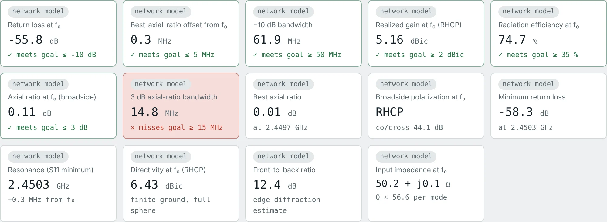
Problem: The corner-truncated CP patch has a −10 dB impedance bandwidth of 61.9 MHz and a 3 dB axial-ratio bandwidth of 14.8 MHz, both centred near 2.45 GHz. What is its usable bandwidth for a CP application?

{BW}_{usable} = \min (61.9, 14.8) = 14.8 MHz = \frac{14.8}{2450} = 0.60 %

Answer: 14.8 MHz (0.60%), set by the axial ratio

Too narrow for the full 83.5 MHz ISM band but plenty for a single GNSS signal (GPS L1 is 2 MHz wide). Dual-feed CP patches with a 90° hybrid extend the AR bandwidth to roughly the impedance bandwidth.

Calculator goal readouts for the CP patch: return loss minus 55.8 dB, minus 10 dB bandwidth 61.9 megahertz, realized gain 5.16 dBic, efficiency 74.7 percent, axial ratio 0.11 dB, 3 dB axial-ratio bandwidth 14.8 megahertz missing a 15 megahertz goal — The CP patch readouts: every goal is met except the 3 dB axial-ratio bandwidth (14.8 MHz against a 15 MHz goal). Try it in the Patch Antenna Calculator →

Doubling the Substrate Thickness

Problem: Using the patch formula, what happens to the bandwidth of the Rogers patch if two 1.524 mm boards are stacked (h = 3.048 mm)? What else changes?

FBW \propto h \Rightarrow 1.19 % \times 2 \approx 2.4 %

Answer: about 2.4% (59 MHz) — enough for the whole 2.4 GHz ISM band

Lower Q also raises efficiency (Part 9). The costs: a larger inset or probe inductance to match, slightly more surface-wave loss, and a higher cross-polarization level from the thicker substrate.

Sizing a Frequency-Independent Antenna

Problem: A log-periodic dipole array must cover 100–1000 MHz. Its longest element must be about λ/2 at the lowest frequency and its shortest about λ/2 at the highest. Find both element lengths and the ratio bandwidth.

L_{max} \approx \frac{3.0}{2} = 1.5 m L_{min} \approx \frac{0.3}{2} = 0.15 m r = 10 : 1 (FBW = 164 %)

Answer: elements from about 1.5 m down to 0.15 m; 10:1 bandwidth

In practice the elements extend about 10–20% beyond these values so that the "active region" of 3–4 resonant elements is complete at the band edges. Bandwidth comes from geometry, not from a low Q (Part 14).

Summary

An antenna has impedance, pattern, gain and polarization bandwidths; the usable bandwidth is where all requirements hold.
Fractional bandwidth (f_H − f_L)/f_c describes narrowband antennas; the ratio f_H:f_L describes broadband ones; FBW = 2(r − 1)/(r + 1).
The −10 dB criterion allows 10% reflected power and 0.46 dB mismatch loss.
Q = 2ω·max(W_e, W_m)/P; for a matched single-resonance antenna FBW = (s − 1)/(Q√s): 0.707/Q for VSWR 2, 0.667/Q at −10 dB.
Loss lowers Q and widens S₁₁ bandwidth — a wide dip is not proof of a good antenna.
The Chu limit Q ≥ 1/(ka)³ + 1/ka bounds small antennas; the Bode–Fano limit bounds what a matching network can add.
Bandwidth is widened by thicker conductors or substrates, lower ε_r, stacked resonances, broadband matching, and travelling-wave or frequency-independent geometries.

The axial-ratio bandwidth of the CP patch introduced a new requirement: the orientation of the field. Part 11: Antenna Polarization covers linear, circular and elliptical polarization, the axial ratio and the polarization loss factor.

Put It Into Practice

Use the NEXT ANTENNAS calculators to apply the ideas from this article to real antennas.

Antenna Design Patch Antenna Calculator Microstrip patch synthesis and simulation: dimensions, feed, S11, gain, efficiency and radiation patterns. Open calculator → Wire Antennas Dipole & Monopole Antenna Calculator Method of Moments design of dipoles, inverted-Vs and monopoles: length, impedance, S11, current, gain and 3D patterns. Open calculator → Link & Power VSWR & Return Loss Calculator Convert between VSWR, return loss, reflection coefficient and mismatch loss. Open calculator → All Tools All RF Calculators Browse every NEXT ANTENNAS calculator for RF, microwave and antenna design. Open calculator →

Antenna Bandwidth and Quality Factor