Antenna Types and Classification

Fig 1 — A map of antenna families by how they radiate. Many practical antennas combine families: a patch array, a horn-fed reflector, a Yagi of dipoles

Introduction to Antenna Classification

Parts 1–13 developed the language every antenna is described in: radiation pattern and beamwidth, directivity and gain, input impedance, efficiency, bandwidth and Q, polarization, effective aperture and the Friis link. This part applies that language to the antennas engineers actually build. The classification follows the mechanism of radiation, because the mechanism decides the trade-offs: a resonant antenna is compact but narrowband (Part 10), an aperture is efficient and high-gain but large in wavelengths (Part 12), and a frequency-independent antenna is wideband but bigger than a resonant one at its lowest frequency.

Practical design details for many of these types are collected in our Antenna Types learning path; the calculators linked at the end let you synthesize dipoles, monopoles and patches directly.

Wire Antennas

Wire antennas carry a current along thin conductors: the current distribution sets the pattern through the radiation integral (Part 2), and the standing wave on the wire sets the impedance (Part 7). They are cheap, light and well understood, and they dominate below about 1 GHz.

Dipole antennas

The centre-fed half-wave dipole is the reference antenna of radio engineering. Its key figures, derived earlier in this series, are:

Property	Half-wave dipole	Derived in
Pattern	cos(π/2·cos θ)/sin θ; HPBW 78°	Part 4
Directivity	1.64 (2.15 dBi)	Part 6
Input impedance (exact λ/2)	73.1 + j42.5 Ω; resonant at 0.47–0.49 λ	Part 7
Effective length / aperture	λ/π; 0.13 λ²	Part 12
Bandwidth (VSWR 2, thin wire)	5–10%	Part 10

Variants change the impedance or the bandwidth: the folded dipole (≈ 292 Ω, a built-in 4:1 transformer, Part 7), the inverted-V (arms drooping 30–60°, lower impedance), the off-centre-fed dipole (multiband operation), and fat or biconical dipoles (lower Q, wider bandwidth).

Monopole antennas

A monopole over a ground plane is half a dipole plus its image (Part 2). A quarter-wave monopole on a large ground has Z ≈ 36 Ω and 5.15 dBi directivity, with its maximum on the horizon and a null overhead — ideal for vehicles, broadcast towers and base-station whips. On a finite ground the beam tilts upward and some current flows on the ground and the cable.

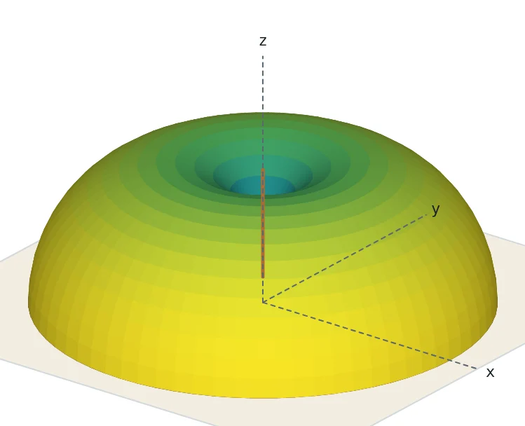
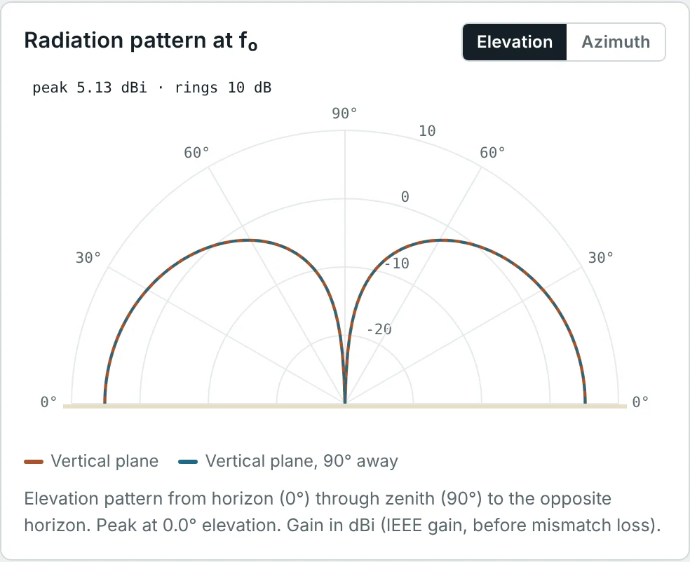
Three-dimensional pattern of a quarter-wave monopole on a ground plane: a half doughnut with a deep null overhead — A 146 MHz quarter-wave monopole on an ideal ground: the upper half of a dipole doughnut, 5.13 dBi on the horizon, null overhead. Try it in the Dipole & Monopole Antenna Calculator →

Elevation pattern of the monopole with the maximum at zero degrees elevation — Its elevation cut: maximum along the ground plane, falling to a null at the zenith. Try it in the Dipole & Monopole Antenna Calculator →

Compact derivatives are everywhere in consumer devices. The inverted-F antenna (IFA) folds the monopole parallel to the ground and adds a short-circuit stub near the feed to bring the impedance to 50 Ω; the planar inverted-F antenna (PIFA) widens the arm into a plate to lower Q. Both are about λ/4 long but only λ/20–λ/10 high. Top-loading with a capacity hat raises the effective height of a short monopole towards its physical height (Part 12).

Loop antennas

Small loops (circumference below about λ/10) are magnetic dipoles: uniform current, sin θ pattern with a null along the loop axis, D = 1.5, and a tiny radiation resistance R_r = 31 200 (NA/λ²)² for N turns. They are poor transmitters but excellent direction-finding and low-noise receiving antennas (the AM ferrite rod), and they are the coupling element of NFC and wireless charging (Part 3). Resonant loops with a circumference of about one wavelength (the "quad" element) have their maximum radiation along the loop axis, about 3.1 dBi directivity and an input impedance of 100–130 Ω.

Aperture Antennas

Aperture antennas radiate from an opening in a guiding structure. The far field is the Fourier transform of the field across the aperture — the same integral as Part 2 with an aperture field in place of a wire current — so the beamwidth scales as λ/D and the directivity as 4πA_eff/λ² (Part 12).

Horn antennas

A horn flares a waveguide gradually into a larger aperture, matching the 377 Ω of free space over a wide band (typically 1.5:1 to 2:1 for standard-gain horns, 10:1 or more for ridged horns). Because the field across the mouth has a quadratic phase error from the flare (the same quantity as the Fresnel-region phase error of Part 3), each horn length has an optimum aperture. The optimum-gain pyramidal horn has an aperture efficiency of about 51%:

Gain and beamwidths of an optimum pyramidal horn (aperture A × B)

G \approx ε_{ap} \frac{4 π A B}{λ^{2}}, ε_{ap} \approx 0.51 {HPBW}_{E} \approx 56 ° \frac{λ}{B} {HPBW}_{H} \approx 67 ° \frac{λ}{A}

A is the H-plane (wide) dimension, B the E-plane dimension. The H-plane field has a cosine taper, hence the wider beam constant. Horns are the standard-gain references used in the gain-transfer measurements of Part 6.

Slot antennas

A narrow slot cut in a conducting sheet is the electromagnetic complement of a strip dipole of the same shape. Babinet's principle, extended to antennas by Booker, links their impedances:

Booker's relation for complementary antennas

Z_{slot} Z_{dipole} = \frac{η^{2}}{4} \approx 35 500 Ω²

The slot's E-field lies across the slot, so its polarization is rotated 90° relative to the complementary dipole; its pattern is otherwise the same (with a sign change on the two sides of the sheet). Slots fed by waveguides form the slotted-waveguide arrays used in radar and aircraft.

Microstrip Patch Antennas

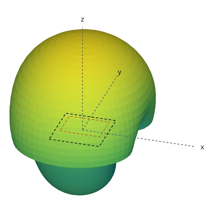
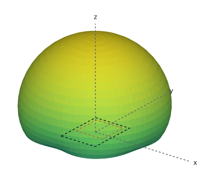
A patch is a metal rectangle on a grounded dielectric substrate. It behaves as a cavity resonator, half a guided wavelength long, whose fringing fields at the two open ends radiate like two slots (Part 2). It is low-profile, cheap to print, easy to array and easy to make circularly polarized (Part 11) — and narrowband (Part 10) and, on lossy substrates, inefficient (Part 9). The standard transmission-line design equations are:

Rectangular patch design equations (Hammerstad / Bahl)

W = \frac{c}{2 f_{0}} \sqrt{\frac{2}{ε_{r} + 1}} ε_{eff} = \frac{ε_{r} + 1}{2} + \frac{ε_{r} - 1}{2} {(1 + 12 \frac{h}{W})}^{- 1 / 2}

Δ L = 0.412 h \frac{(ε_{eff} + 0.3) (W / h + 0.264)}{(ε_{eff} - 0.258) (W / h + 0.8)} L = \frac{c}{2 f_{0} \sqrt{ε_{eff}}} - 2 Δ L

W is chosen for good radiation efficiency; L sets the resonant frequency. ΔL is the electrical extension caused by fringing at each open end. The edge resistance (150–400 Ω) is brought to 50 Ω with an inset feed, a quarter-wave transformer or a probe placed inside the patch.

Three-dimensional pattern of a 2.45 gigahertz patch: a broad lobe above the ground plane and a small back lobe — A 2.45 GHz linearly polarized patch: one broad beam above the board, 6–7 dBi directivity. Try it in the Patch Antenna Calculator →

Three-dimensional realized gain pattern of the corner-truncated circularly polarized patch — The corner-truncated RHCP patch of Part 11: a similar broad dome, now 5.2 dBic realized gain in circular polarization. Try it in the Patch Antenna Calculator →

Reflector Antennas

A reflector antenna uses a large conducting surface, illuminated by a small feed, to produce a large, nearly uniform aperture. It is the most economical way to obtain very high gain (30–70 dBi).

Parabolic reflector antennas

A paraboloid has the property that every ray from its focus, after reflection, travels parallel to the axis, and every path from the focus to a plane across the aperture has the same length. A spherical wave from a feed at the focus therefore becomes a plane wave across the aperture:

Parabola, equal path lengths, and dish performance

ρ^{2} = 4 f z r (ψ) + r (ψ) \cos ψ = 2 f G = ε_{ap} {(\frac{π D}{λ})}^{2} HPBW \approx 70 ° \frac{λ}{D}

f is the focal length, ψ the angle from the axis at the focus. The second relation states that the path focus → reflector → aperture plane is 2f for every ray. The gain formula is the aperture formula of Part 12 for a circle of diameter D. The f/D ratio (0.25–0.6 for prime focus) sets how much the feed pattern must taper.

Dual-reflector systems (Cassegrain with a hyperboloidal sub-reflector, Gregorian with an ellipsoidal one) put the feed behind the main dish, shorten the structure and allow shaped surfaces with aperture efficiencies of 75–85%. Offset reflectors move the feed out of the beam to remove blockage — the design of most consumer satellite dishes.

Corner reflector antennas

A dipole placed in front of two conducting sheets meeting at 90° produces, by image theory, three image dipoles. The four-element array gives 10–12 dBi with a simple, robust structure, popular for UHF TV and point-to-point links. The spacing of the dipole from the apex (about 0.5 λ) controls gain and impedance.

Helical Antennas

A conductor wound into a helix of diameter D, circumference C = πD, turn spacing S and N turns radiates in two very different modes:

Normal mode (C ≪ λ): the helix behaves like a short dipole plus a small loop; the pattern is broadside and the polarization elliptical. Used as compact "rubber duck" whips on handheld radios.
Axial mode (3/4 < C/λ < 4/3): a travelling wave runs along the helix and the beam points along its axis, circularly polarized. Kraus's empirical design formulas are:

Axial-mode helix (Kraus), valid for 12° ≤ pitch angle ≤ 14°, N > 3

D_{0} \approx 15 N \frac{C^{2} S}{λ^{3}} HPBW \approx \frac{52 ° λ^{3 / 2}}{C \sqrt{N S}} R_{in} \approx 140 \frac{C}{λ} Ω AR \approx \frac{2 N + 1}{2 N}

The sense of circular polarization follows the sense of the winding. Later measurements show the directivity formula over-estimates by 2–3 dB for long helices, but the trends are right: gain grows with axial length NS. Bandwidth is about 1.7:1.

Spiral Antennas

Rumsey observed that an antenna whose shape is defined entirely by angles has no characteristic length, and so its properties cannot change with frequency. The equiangular (log) spiral, r = r₀e^(aφ), is such a shape; truncating it at an outer radius sets the lowest frequency, and the feed region sets the highest. The Archimedean spiral, r = r₀ + aφ, is not strictly self-scaling but behaves similarly. Radiation comes from an "active region" where the arm circumference is about one wavelength; as frequency changes, that region moves inward or outward.

Mushiake's relation for self-complementary antennas

Z_{in} = \frac{η}{2} \approx 188.5 Ω at all frequencies

When the metal and the gaps have identical shapes, Booker's relation (above) with Z_slot = Z_metal gives Z² = η²/4. Two-arm self-complementary spirals have input impedances of 150–190 Ω, fed through a broadband balun. Spirals radiate circular polarization with bandwidths of 10:1 to 40:1 and are widely used in electronic warfare and direction finding.

Yagi-Uda Antennas

A Yagi-Uda antenna has one driven element (usually a dipole or folded dipole), a slightly longer reflector behind it and several slightly shorter directors in front. The parasitic elements are not fed; they are excited by mutual coupling. A longer-than-resonant element is inductive, so its current lags and it re-radiates in a way that reinforces radiation away from it; a shorter element is capacitive, its current leads, and it pulls the beam toward itself. The result is an end-fire array with a phase progression close to that of a travelling wave along the boom.

Elements	Typical boom length	Gain	Front-to-back
2 (driven + reflector)	0.1–0.2 λ	≈ 6–7 dBi	10–15 dB
3	0.25–0.4 λ	≈ 7–9 dBi	15–25 dB
6	≈ 1 λ	≈ 10–12 dBi	20–25 dB
15	≈ 4 λ	≈ 14–16 dBi	20–30 dB

Gain grows roughly 2.5–3 dB per doubling of boom length; adding directors to a short boom helps little. Mutual coupling lowers the driven element's impedance to 10–30 Ω, which is why Yagis often use a folded dipole or a gamma or hairpin match (Part 8). Their bandwidth is modest (a few percent for high-gain designs).

Log-Periodic Antennas

A log-periodic dipole array (LPDA) is a row of dipoles whose lengths and spacings shrink by a constant ratio τ from back to front, fed by a transmission line that is crossed between adjacent elements. At any frequency, the three or four elements near λ/2 long form an "active region" that radiates toward the short end, while longer elements behave as reflectors and shorter ones as directors. Moving the frequency moves the active region; the pattern and impedance repeat periodically with the logarithm of frequency, with period ln(1/τ). Carrel's design relations are:

LPDA design (Carrel)

τ = \frac{L_{n + 1}}{L_{n}} = \frac{R_{n + 1}}{R_{n}} σ = \frac{d_{n}}{2 L_{n}} \tan α = \frac{1 - τ}{4 σ}

B_{ar} = 1.1 + 7.7 {(1 - τ)}^{2} \cot α B_{s} = B B_{ar} N = 1 + \frac{\ln B_{s}}{\ln (1 / τ)}

R_n is the distance of element n from the apex, d_n the spacing, α the half-angle of the array's outline. B is the required bandwidth ratio, B_ar the width of the active region and B_s the structure bandwidth that the element lengths must span. τ ≈ 0.8–0.95 and σ ≈ 0.05–0.2 give 6.5–10.5 dBi.

Dielectric Resonator Antennas

A dielectric resonator antenna (DRA) is a block of low-loss, high-permittivity ceramic (ε_r ≈ 10–40) on a ground plane, excited by a probe, a slot or a microstrip line. Its resonant modes radiate because, unlike a closed cavity, the dielectric boundary lets fields leak out. With no metal in the radiating structure, DRAs have no conductor loss and high efficiency even at millimetre-wave frequencies, and their bandwidth (5–15%) is wider than a patch's. For the HEM₁₁δ mode of a cylindrical DRA of radius a and height h, an accurate empirical formula (Mongia and Bhartia) is

Resonant frequency of a cylindrical DRA (HEM₁₁δ mode, broadside radiation)

f_{0} = \frac{6.324 c}{2 π a \sqrt{ε_{r} + 2}} [0.27 + 0.36 \frac{a}{2 h} + 0.02 {(\frac{a}{2 h})}^{2}]

Valid for 0.4 ≤ a/h ≤ 6. The resonator's size scales roughly as λ₀/√ε_r, and its Q falls as ε_r decreases, trading size against bandwidth exactly as the Chu limit predicts (Part 10).

Travelling-Wave Antennas

If a long wire is terminated in its characteristic impedance instead of being left open, the current is a single wave travelling toward the termination rather than a standing wave. Without reflections, the impedance is nearly constant over a wide band. The radiation of a wire of length L carrying a travelling wave forms a cone of lobes tilted toward the far end; the main lobe is at

Main-lobe angle of a terminated long wire

θ_{m} \approx \cos^{- 1} (1 - \frac{0.371 λ}{L})

θ_m is measured from the wire. Longer wires radiate closer to their axis. Pairs of wires arranged as a V or a rhombus combine these cones into a single high-gain beam, the basis of the classic HF rhombic and of the low-noise Beverage receiving antenna.

Other travelling-wave antennas include the axial-mode helix (above), dielectric-rod and Yagi-like surface-wave antennas, leaky-wave antennas whose beam scans with frequency, and the tapered-slot Vivaldi antenna, in which a wave travels along an exponentially widening slot until it detaches — giving 10:1 bandwidths in a flat printed form.

Broadband and Ultra-Wideband Antennas

Broadband antennas avoid a single high-Q resonance (Part 10) by one of four routes: fat or flared conductors (biconical, bowtie, discone, planar disc monopoles), self-scaling geometry (log-periodic, spiral), travelling-wave operation (Vivaldi, horn, helix) or overlapping resonances (stacked and multi-branch structures). For impulse-radio UWB (3.1–10.6 GHz), the antenna must also preserve the shape of a nanosecond pulse: a stable phase centre and low group-delay variation matter as much as S₁₁. Planar elliptical monopoles and small Vivaldis are the common choices.

Modern and Reconfigurable Antennas

Technology	What it does	Typical use
Frequency-reconfigurable antennas	PIN diodes, RF switches or varactors change the electrical length or the matching	Smartphones covering many LTE/5G bands with a small antenna (overcoming the Chu limit by tuning)
Pattern- and polarization-reconfigurable antennas	Switch parasitic elements or feed points to steer the beam or change polarization	Wi-Fi access points, IoT gateways
Phased arrays and massive MIMO	Electronic amplitude and phase control of many elements (Part 4)	5G base stations (64T64R), radar, satellite user terminals
Antenna-in-package (AiP)	Antenna arrays integrated with the RF chip in one package	28/39/60 GHz phones and modules
Metasurfaces and reconfigurable intelligent surfaces	Engineered sub-wavelength scatterers shape reflected or transmitted waves	Thin reflectarrays, transmitarrays, coverage enhancement
Fractal and meandered antennas	Space-filling geometries fit a long current path into a small area; multi-band self-similarity	Compact multiband IoT antennas
Wearable, flexible and liquid-metal antennas	Textile or stretchable conductors; reshaping to retune	Body-area networks, medical sensors

Comparing Antenna Types

Type	Gain	Bandwidth	Polarization	Size	Typical band
Half-wave dipole	2.15 dBi	5–10%	Linear	λ/2	HF–UHF
λ/4 monopole	5.15 dBi (ideal ground)	8–12%	Linear (vertical)	λ/4 + ground	MF–UHF
Small loop	1.76 dBi (directivity), low gain	< 1%	Linear	< λ/10	LF–HF, NFC
Patch	5–8 dBi	1–5% (up to 30% broadbanded)	Linear or CP	≈ λ/2√ε_r, flat	0.5–100 GHz
Yagi-Uda	7–16 dBi	2–10%	Linear	0.2–4 λ boom	HF–UHF
Log-periodic	6.5–10.5 dBi	2:1–20:1	Linear	≈ λ_max/2 wide	HF–microwave
Axial-mode helix	10–16 dBi	≈ 1.7:1	Circular	C ≈ λ, length NS	UHF–S band
Spiral	2–5 dBi	10:1–40:1	Circular	Diameter ≈ λ_max/π	0.5–40 GHz
Horn	10–25 dBi	1.5:1–10:1	Linear (or CP with polarizer)	Several λ	1–300 GHz
Parabolic reflector	25–70 dBi	Set by the feed	Any	10–1000 λ	1–300 GHz
DRA	5–8 dBi	5–15%	Linear or CP	≈ λ/√ε_r	1–100 GHz
Vivaldi	5–12 dBi	5:1–10:1	Linear	≈ λ_max/2 long	1–40 GHz

Worked Examples

Designing a 2.45 GHz Patch on FR-4

Problem: Find W, ε_eff, ΔL and L for a rectangular patch at 2.45 GHz on FR-4 (ε_r = 4.3, h = 1.6 mm), and compare with the Patch Calculator's 37.58 × 29.30 mm.

W = 61.18 \sqrt{\frac{2}{5.3}} = 37.58 mm ε_{eff} = 2.65 + 1.65 {(1.511)}^{- 0.5} = 3.99 Δ L = 0.74 mm

L = \frac{61.18}{\sqrt{3.99}} - 2 (0.74) = 30.62 - 1.48 = 29.14 mm

Answer: W = 37.58 mm, L = 29.14 mm — the calculator's refined design is 29.30 mm

The closed-form equations land within 0.6% of the calculator, which then refines the length with a field solver and dispersion correction. That accuracy matters: a 1% length error moves the resonance by 25 MHz, a third of the bandwidth.

Impedance of a Half-Wave Slot

Problem: Use Booker's relation to find the impedance of a half-wave slot whose complementary strip dipole has Z = 73.1 + j42.5 Ω.

Z_{slot} = \frac{35}{} = \frac{35 530 (73.1 - j 42.5)}{7150} = 363 - j 211 Ω

Answer: 363 − j211 Ω

A dipole that is slightly inductive has a complementary slot that is capacitive. A centre-fed slot is a high-impedance antenna; it is fed off-centre or with a microstrip line crossing it to reach 50 Ω.

Gain of a Standard-Gain Horn

Problem: A 10 GHz optimum pyramidal horn has a 15 cm × 10 cm mouth. Estimate its gain and beamwidths.

G = 0.51 \frac{4 π (0.15) (0.10)}{{0.03}^{2}} = 107 = 20.3 dBi {HPBW}_{E} \approx 56 ° \times 0.3 = 16.8 ° {HPBW}_{H} \approx 67 ° \times 0.2 = 13.4 °

Answer: about 20.3 dBi, with beamwidths of about 17° (E-plane) and 13° (H-plane)

Check with Kraus (Part 6): 41 253/(16.8 × 13.4) = 183 = 22.6 dBi — an overestimate, as expected for real beams with tapered edges.

Beamwidth of a Satellite Dish

Problem: A 1.2 m dish at 12 GHz has a gain of 41.7 dBi (Part 12). Estimate its HPBW and the pointing accuracy needed to stay within 1 dB of peak (−1 dB is about 0.29 of the 3 dB beamwidth from the axis).

HPBW \approx 70 ° \frac{0.025}{1.2} = 1.46 ° Δ θ_{1 dB} \approx 0.29 \times 1.46 ° = 0.42 °

Answer: HPBW ≈ 1.5°; the dish must be aimed within about ±0.4°

The −1 dB offset follows from the parabolic approximation of the main lobe, loss(dB) ≈ 12(Δθ/HPBW)². High gain always comes with tight pointing requirements.

An L-Band Axial-Mode Helix

Problem: Design a 10-turn axial-mode helix for 1.6 GHz with C = λ and a 13° pitch angle. Estimate D, HPBW, R_in and AR with Kraus's formulas.

λ = 18.74 cm, D = \frac{C}{π} = 5.97 cm, S = C \tan 13 ° = 4.33 cm = 0.231 λ

D_{0} = 15 \times 10 \times 0.231 = 34.6 = 15.4 dBi HPBW = \frac{52}{\sqrt{2.31}} = 34 ° R_{in} \approx 140 Ω AR = \frac{21}{20} = 0.42 dB

Answer: 6 cm diameter, 43 cm long; about 15 dBi (Kraus; 12–13 dBi in modern measurements), 34° beam, 140 Ω, AR 0.4 dB

A tapered first turn or a strip-line section transforms 140 Ω to 50 Ω. Winding direction sets RHCP or LHCP.

How Many Elements Does an LPDA Need?

Problem: Design an LPDA for 100–1000 MHz with τ = 0.9 and σ = 0.15. Find α, B_ar, B_s and N.

α = \tan^{- 1} \frac{0.1}{0.6} = 9.46 ° B_{ar} = 1.1 + 7.7 (0.01) (6.00) = 1.56 B_{s} = 15.6 N = 1 + \frac{\ln 15.6}{\ln (1.111)} = 27.1

Answer: 28 elements, with the longest about 1.5 m and an outline half-angle of 9.5°

The longest element is λ_max/2 = 1.5 m and each next one is 0.9 times shorter. τ = 0.9 with σ = 0.15 gives roughly 8.5 dBi; a larger τ (closer to 1) gives more gain but needs more elements.

First-Cut Yagi Element Lengths

Problem: Estimate first-cut element lengths and spacing for a 3-element 146 MHz Yagi: driven element 0.47 λ, reflector 5% longer, director 5% shorter, spacings 0.2 λ.

L_{DE} = 0.47 \times 2.053 = 0.965 m L_{R} = 1.013 m L_{D} = 0.917 m s = 0.41 m

Answer: reflector 1.01 m, driven element 0.97 m, director 0.92 m, 0.41 m apart (0.82 m boom)

Expect about 7–8 dBi and a driven-element impedance of 20–30 Ω; a hairpin or gamma match (Part 8) brings it to 50 Ω. Real designs are optimized numerically — mutual coupling makes the lengths interact.

Resonant Frequency of a Cylindrical DRA

Problem: A cylindrical DRA has ε_r = 10, radius a = 6 mm and height h = 6 mm. Find the HEM₁₁δ resonant frequency.

\frac{a}{2 h} = 0.5 f_{0} = \frac{6.324 \times 3 \times 10^{8}}{2 π (0.006) \sqrt{12}} (0.27 + 0.18 + 0.005) = 6.6 GHz

Answer: about 6.6 GHz

The resonator is 12 mm across, about 0.26 λ₀ — a little over half the size of an air patch, with no conductor loss. Raising ε_r to 20 would shrink it further at the cost of bandwidth.

Main Lobe of a Long-Wire Antenna

Problem: A terminated long wire is 5 λ long. At what angle from the wire is its main lobe?

θ_{m} = \cos^{- 1} (1 - \frac{0.371}{5}) = \cos^{- 1} (0.926) = 22.2 °

Answer: about 22° from the wire, toward the terminated end

A V antenna with each leg 5 λ long and an included angle of about 2 × 22° = 44° lines up one lobe from each leg along the bisector, adding them into a single beam.

Feeding a One-Wavelength Loop

Problem: A square one-wavelength loop for 14.2 MHz has an input resistance of about 110 Ω. Find its side length and design a quarter-wave transformer to 50 Ω using coax with a velocity factor of 0.66.

λ = 21.1 m \Rightarrow side \approx \frac{λ}{4} = 5.28 m Z_{T} = \sqrt{50 \times 110} = 74 Ω ℓ = 0.66 \times \frac{21.1}{4} = 3.48 m

Answer: 5.3 m sides; a 3.48 m section of 75 Ω coax matches it to 50 Ω

Standard 75 Ω cable is almost exactly the required 74 Ω — a lucky coincidence that made the "quad" popular. The loop is resonant when its perimeter is slightly more than λ (about 1.02 λ in practice).

Summary

Antennas are classified by how they radiate: resonant wire, slot, patch and dielectric antennas; aperture and reflector antennas; and travelling-wave or frequency-independent antennas.
Dipoles (2.15 dBi, 73 Ω) and monopoles (5.15 dBi, 36 Ω on ideal ground) remain the workhorses below 1 GHz; IFAs and PIFAs bring them into devices.
Horns (G ≈ 0.51·4πAB/λ²) and reflectors (G = ε_ap(πD/λ)², HPBW ≈ 70°λ/D) provide high gain; slots are Babinet duals of dipoles, Z_slot Z_dipole = η²/4.
Patches are designed with W, ε_eff, ΔL and L formulas that land within about 1% of full-wave results; they are flat, CP-capable and narrowband.
Axial-mode helices give circularly polarized beams; spirals and log-periodic arrays give 10:1 or more bandwidth from angle-defined or self-scaling geometry; self-complementary antennas have Z = 188.5 Ω.
Yagi-Uda arrays use parasitic reflectors and directors for 7–16 dBi; DRAs avoid conductor loss; travelling-wave antennas trade size for bandwidth.
Modern antennas add reconfigurability, beam steering and integration — but every one of them is still described by the pattern, gain, impedance, efficiency, bandwidth, polarization and aperture developed in this series.

This completes the Antenna Fundamentals series. To keep going, explore our Antenna Types learning path for practical designs, the Smith Chart & Impedance Matching series for matching, and the Maxwell's Equations series for the field theory underneath it all. Or return to the series overview.

Put It Into Practice

Use the NEXT ANTENNAS calculators to apply the ideas from this article to real antennas.

Wire Antennas Dipole & Monopole Antenna Calculator Method of Moments design of dipoles, inverted-Vs and monopoles: length, impedance, S11, current, gain and 3D patterns. Open calculator → Wire Antennas Monopole & Ground Plane Calculator Quarter-wave monopoles and ground-plane antennas with radials: length, impedance and radial angle. Open calculator → Antenna Design Patch Antenna Calculator Microstrip patch synthesis and simulation: dimensions, feed, S11, gain, efficiency and radiation patterns. Open calculator → All Tools All RF Calculators Browse every NEXT ANTENNAS calculator for RF, microwave and antenna design. Open calculator →