Antenna Radiation Patterns Explained

3D radiation pattern of a half-wave dipole: a doughnut-shaped surface around a horizontal wire, with a deep null along the wire axis — The 3D radiation pattern of a half-wave dipole at 146 MHz, solved with the Method of Moments. The surface is a doughnut around the wire: strong broadside, falling to a null along the wire axis (the dimple on the left). Both radius and colour show gain, from 30 dB below the 2.12 dBi peak up to the peak. Try it in the Dipole & Monopole Antenna Calculator →

What Is an Antenna Radiation Pattern?

No real antenna radiates equally in all directions. A radiation pattern is a graph of how the radiated field (or power) varies with direction, measured at a fixed, large distance from the antenna. It answers the most practical question about any antenna: where does the energy go?

Direction is described with spherical coordinates centred on the antenna: the elevation angle θ measured from the z-axis and the azimuth angle φ measured around it. The pattern is defined in the far field, where its shape no longer changes with distance — Part 3 explains why that matters. By reciprocity, the same pattern describes how well the antenna receives from each direction.

Shape, not sizeA pattern is usually normalised so that its maximum is 0 dB (or 1). It shows relative levels; gain (Part 6) sets the absolute scale.

Field or powerField patterns plot |E|; power patterns plot |E|². In decibels the two are identical.

Transmit = receiveFor passive antennas, reciprocity makes the transmit and receive patterns the same.

Coordinates and the Normalized Pattern

Antenna engineers use a spherical coordinate system centred on the antenna. A direction is given by two angles: θ, measured down from the z-axis (0° to 180°), and φ, measured around the z-axis from the x-axis (0° to 360°). The far-field electric field has only two components, E_θ and E_φ, both perpendicular to the direction of travel.

Fig 1 — Spherical coordinates used for radiation patterns: θ from the z-axis, φ in the xy-plane from the x-axis

In the far field every component falls off as e^−jkr/r, so the field can be written as a distance term times a purely angular term. That angular term, scaled to a maximum of 1, is the normalized field pattern:

Normalized field and power patterns

F (θ, φ) = \frac{| E (r, θ, φ) |}{| E |_{max}} P_{n} (θ, φ) = F^{2} (θ, φ) P_{dB} = 20 \log_{10} F = 10 \log_{10} P_{n}

F is independent of r in the far field. The power pattern P_n is proportional to the radiation intensity U(θ, φ) of Part 5, which is why the same function appears again in the directivity integral of Part 6.

Radiation Pattern Representation

The same pattern can be drawn in several ways. Each makes different features easy to see:

Fig 2 — One pattern, three scales: the half-wave dipole in a cut containing the wire (wire along 0°–180°)

Linear field |E|

Linear power |E|²

Logarithmic, dB

Representation	What is plotted	Best for
Field pattern (linear)	\|E(θ, φ)\| / \|E\|max	Seeing the main beam shape; −3 dB point at 0.707
Power pattern (linear)	\|E\|² / \|E\|²max	Seeing where the power goes; −3 dB point at 0.5
Decibel pattern	20 log₁₀\|E\|/\|E\|max	Side lobes, back lobes and nulls — small levels become visible
Gain pattern (dBi)	G(θ, φ) in dBi	Link budgets: shows absolute gain in every direction

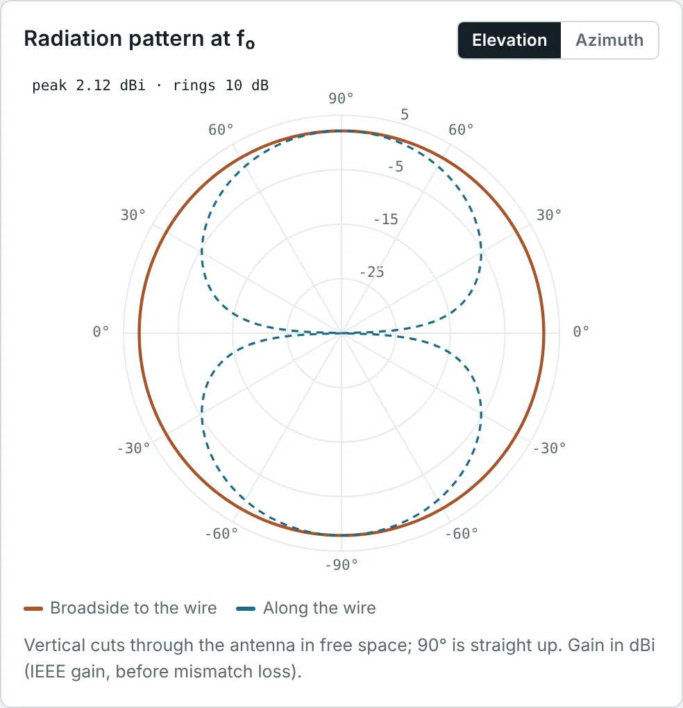
Because 20 log|E| and 10 log|E|² are the same number, a dB pattern is the same whether it started from field or power. Most datasheets and simulators therefore plot in dB, with rings every 10 dB, as in the calculator screenshots below. If decibels are new to you, see our guide to dB, dBm and dBi.

Where a Radiation Pattern Comes From

A pattern is not something we have to measure to know: it follows directly from the current on the antenna. The procedure is always the same — find the magnetic vector potential A produced by the current, keep only the terms that fall off as 1/r, and read off the angular dependence. We do it here for the three building blocks of antenna theory. The field equations themselves are developed in Part 10 of our Maxwell's Equations series.

Pattern of a Hertzian (Short) Dipole

Take a very short current element of length L ≪ λ along the z-axis, carrying a uniform current I. Its vector potential at distance r is

Step 1 — vector potential of a current element

A = \hat{z} \frac{μ I L}{4 π r} e^{- j k r} A_{θ} = - A_{z} \sin θ

k = 2π/λ is the wavenumber. Projecting ẑ onto the spherical unit vectors gives ẑ = r̂ cos θ − θ̂ sin θ, so the θ-component of A carries a factor −sin θ.

In the far field the electric field is simply −jω times the transverse part of A (the r̂-component does not radiate):

Step 2 — far field of the Hertzian dipole

E_{θ} \approx - j ω A_{θ} = j η \frac{k I L}{4 π r} e^{- j k r} \sin θ H_{φ} = \frac{E_{θ}}{η}

ωμ = ηk, with η = √(μ/ε) ≈ 377 Ω in free space. All the angular dependence is in the factor sin θ.

Step 3 — the normalized pattern

F_{short} (θ) = \sin θ

Maximum broadside (θ = 90°), nulls along the wire (θ = 0° and 180°), and no dependence on φ: the doughnut of the hero figure.

Pattern of a Half-Wave Dipole

A practical dipole is not short, so the current varies along it. For a thin centre-fed dipole of total length λ/2 the current is close to a standing wave that is maximum at the feed and zero at the tips: I(z′) = I₀ cos(kz′) for |z′| ≤ λ/4. Each piece dz′ is a Hertzian dipole; in the far field its distance to the observer is r − z′ cos θ, which shifts its phase by e^{+jkz′ cos θ}. Adding them up:

Superposing the current elements

E_{θ} = j η \frac{k e^{- j k r}}{4 π r} \sin θ \int_{- λ / 4}^{λ / 4} I_{0} \cos (k z^{'}) e^{j k z^{'} \cos θ} d z^{'}

The integrand's imaginary part is odd and vanishes; the real part integrates to (2/k)·cos(π/2 · cos θ)/sin²θ. Substituting:

Far field and pattern of the half-wave dipole

E_{θ} = j η \frac{I_{0} e^{- j k r}}{2 π r} \frac{\cos (\frac{π}{2} \cos θ)}{\sin θ} F_{λ / 2} (θ) = \frac{\cos (\frac{π}{2} \cos θ)}{\sin θ}

The pattern is still a doughnut with nulls along the wire, but slightly flatter than sin θ: the half-power beamwidth drops from 90° to 78.1° (Example 2).

Pattern Multiplication and the Array Factor

Directional antennas are very often arrays of identical elements. If N elements are placed along a line with spacing d and fed with equal amplitudes and a progressive phase β, the far field is the field of one element multiplied by a sum of phase terms. This is the principle of pattern multiplication:

Pattern multiplication

E_{total} = E_{element} \times AF AF = \sum_{n = 0}^{N - 1} e^{j n ψ} ψ = k d \sin θ + β

Here θ is measured from broadside (perpendicular to the array line). ψ is the total phase difference between neighbouring elements: the path difference kd sin θ plus the feed phase β.

The sum is a geometric series, so it has a closed form. Multiplying by (e^jψ − 1), cancelling, and factoring out e^jNψ/2 and e^jψ/2:

Normalized array factor of a uniform linear array

AF = \frac{e^{j N ψ} - 1}{e^{j ψ} - 1} = e^{j (N - 1) ψ / 2} \frac{\sin (N ψ / 2)}{\sin (ψ / 2)} \Rightarrow {AF}_{n} (ψ) = \frac{\sin (N ψ / 2)}{N \sin (ψ / 2)}

AF_n = 1 when ψ = 0 (all elements in phase). Everything that follows — main beam, nulls, side lobes, beamwidth, steering and grating lobes — can be read from this one function.

The directional pattern in the lobe and beamwidth figures below is exactly this: four elements spaced λ/2 (kd = π, β = 0), each with a mildly directional element pattern (1 + 0.6 cos θ)/1.6 so that the back lobe is lower than the main lobe.

Three-Dimensional Radiation Patterns

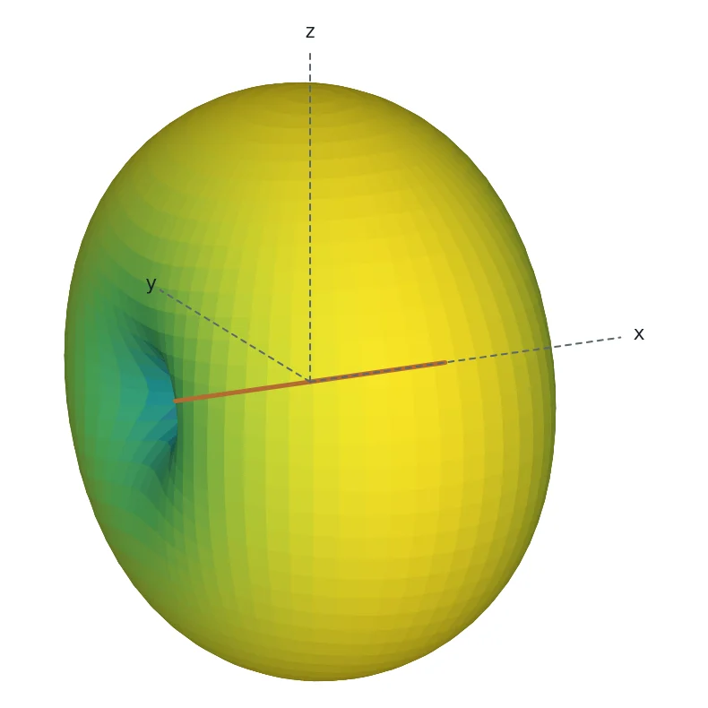
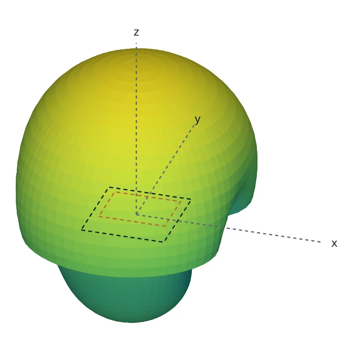
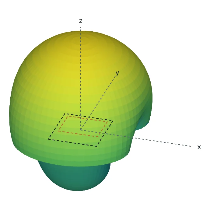
A 3D pattern draws a surface whose distance from the origin is proportional to the radiation in that direction. It gives the complete picture at a glance: the dipole's doughnut above, or the single forward-pointing beam of a microstrip patch below.

3D radiation pattern of a microstrip patch antenna: a broad dome above the board with a smaller lobe below it — A 2.45 GHz microstrip patch on FR-4: one broad beam above the board, and a weaker back lobe below it caused by the finite ground plane. Try it in the Patch Antenna Calculator →

3D radiation pattern of a patch antenna on a Rogers substrate, similar dome with a back lobe — The same design on Rogers RO4003C (1.52 mm). The shape is almost identical; Part 6 shows why its gain is about 3 dB higher. Try it in the Patch Antenna Calculator →

Two-Dimensional Radiation Patterns

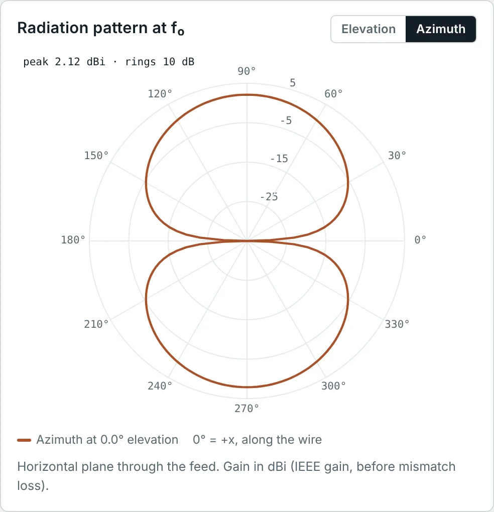
3D surfaces are hard to read numerically, so engineers mostly work with 2D cuts: slices through the 3D pattern along a plane, plotted on a polar chart (angle around the circle, level along the radius) or on a rectangular chart (angle along x, level in dB along y). Two cuts at right angles, through the direction of maximum radiation, describe most antennas well.

Elevation cuts of the dipole: a circle broadside to the wire and a figure-eight along the wire — Elevation cuts of the dipole. Broadside to the wire (orange) the cut is a circle; in the plane containing the wire (blue, dashed) it is a figure-eight with nulls along the wire. Try it in the Dipole & Monopole Antenna Calculator →

Azimuth cut of the horizontal dipole: a figure-eight pattern with nulls at 0 and 180 degrees — The horizontal cut through the same dipole: a figure-eight, peak 2.12 dBi at 90° and 270°, deep nulls at 0° and 180° where the wire points. Try it in the Dipole & Monopole Antenna Calculator →

E-Plane and H-Plane Radiation Patterns

For a linearly polarized antenna, two specific cuts are standard:

E-plane — the plane containing the electric field vector and the direction of maximum radiation.
H-plane — the plane containing the magnetic field vector and the direction of maximum radiation. It is perpendicular to the E-plane.

E-plane and H-plane polar patterns of the FR-4 patch antenna with a broad main lobe at 0 degrees and a back lobe at 180 degrees — E-plane (orange, along the feed) and H-plane (blue) of the FR-4 patch. Both have one broad main lobe pointing away from the board (0°). The E-plane is wider and stays high down to the horizon, because the two radiating slots add up along the feed direction; the H-plane narrows towards ±90°. Try it in the Patch Antenna Calculator →

Principal Plane Patterns

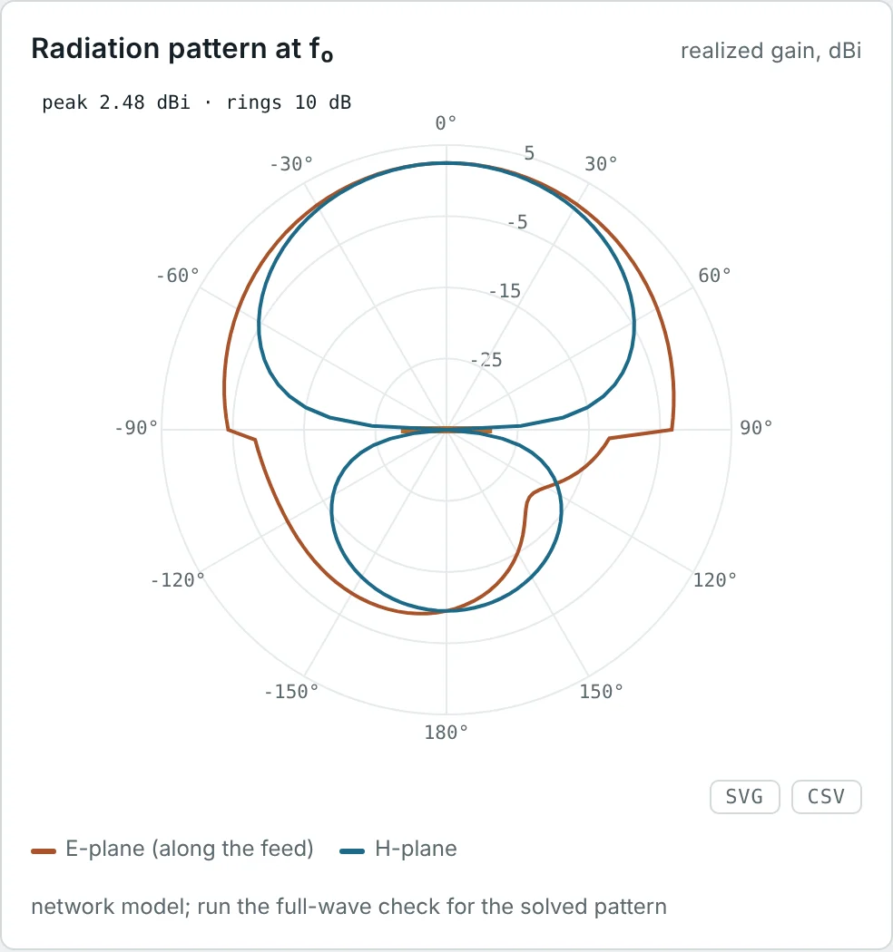
The E- and H-plane cuts are called the principal planes. For most antennas they line up with the coordinate planes, which makes measurements and datasheets consistent:

Antenna (orientation)	E-plane	H-plane	Typical shapes
Vertical dipole or monopole (along z)	Any vertical plane (e.g. xz, φ = 0°)	Horizontal plane (xy, θ = 90°)	E: figure-eight · H: circle
Horizontal dipole (along x)	Horizontal plane containing the wire	Vertical plane broadside to the wire	E: figure-eight · H: circle (in free space)
Patch on xy plane, fed along y	yz plane (along the feed)	xz plane	Both: single broad beam towards +z
Horn, waveguide TE₁₀ (E along y)	yz plane	xz plane	E: narrower · H: wider, lower side lobes

Most antennas also have a third common view: the azimuth cut in the horizontal plane, which is what matters for anything mounted on a mast or a ceiling.

Isotropic, Omnidirectional and Directional Patterns

Fig 3 — The three basic pattern types, each plotted in dB (30 dB range)

Isotropic (reference only)

Omnidirectional (dipole, vertical cut)

Directional (4-element array)

Isotropic Radiation Pattern

An isotropic radiator radiates the same power in every direction: its 3D pattern is a sphere and every cut is a circle. No physical antenna can do this — the transverse nature of electromagnetic waves makes it impossible — but it is the universal reference. Gains quoted in dBi are relative to it.

Omnidirectional Radiation Patterns

An omnidirectional antenna has a non-directional (circular) pattern in one plane and a directional pattern in the perpendicular plane. A vertical dipole or monopole is the classic example: equal coverage in all horizontal directions, nulls straight up and down. This is what Wi-Fi access points, IoT nodes, FM broadcast and mobile phones need — the direction of the other end of the link is unknown or changing.

Directional Radiation Patterns

A directional antenna concentrates its radiation into one main direction. Yagi-Uda antennas, patches, horns, dishes and arrays are all directional. Concentrating the energy gives more range in the wanted direction and less interference in others, at the cost of having to point the antenna.

Main Lobe, Side Lobes and Back Lobe

The pattern of a directional antenna is divided into lobes — regions of radiation separated by nulls or deep minima.

Fig 4 — Lobes of a directional pattern (4-element broadside array with directional elements, d = λ/2)

Lobe	Definition	Why it matters
Main (major) lobe	The lobe containing the direction of maximum radiation	Sets the coverage and the gain
Side lobes	Lobes next to the main lobe, usually in the forward half	Interference and susceptibility to jamming; the side-lobe level (SLL) is quoted relative to the main lobe, e.g. −13 dB
Back lobe	The lobe pointing opposite to the main lobe (≈ 180°)	Radiation behind the antenna, sets the front-to-back ratio
Minor lobes	All lobes except the main lobe — side lobes, back lobe and any others	Wasted power and unwanted coverage

A uniform array of N elements has its first side lobes at about −13 dB for large N; tapering the element amplitudes (Taylor, Chebyshev weighting) lowers them at the cost of a slightly wider main beam.

Half-Power Beamwidth (HPBW)

The half-power beamwidth is the angle between the two directions in the main lobe where the radiated power has fallen to half its maximum: −3 dB, or 0.707 of the maximum field. It is the usual measure of how narrow a beam is, and it is quoted separately for the E-plane and H-plane.

Definition — solve for the half-power angles θ₁ and θ₂ on either side of the peak

F^{2} (θ_{1, 2}) = \frac{1}{2} \Leftrightarrow F (θ_{1, 2}) = \frac{1}{\sqrt{2}} HPBW = | θ_{2} - θ_{1} |

For a simple pattern such as sin θ the equation can be solved by hand; for most patterns it is solved numerically, as in Examples 2 and 5.

HPBW of a Uniform Array

Near the main beam of a broadside array (β = 0, small θ), ψ = kd sin θ is small and sin(ψ/2) ≈ ψ/2, so the normalized array factor becomes the familiar sinc function:

Small-angle form near the main beam

{AF}_{n} \approx \frac{\sin x}{x} x = \frac{N ψ}{2} = \frac{N k d}{2} \sin θ \frac{\sin x}{x} = \frac{1}{\sqrt{2}} \Rightarrow x = 1.3916

So the half-power point is at sin θ_h = 2(1.3916)/(Nkd) = 0.443 λ/(Nd). For a long array θ_h is small, sin θ_h ≈ θ_h, and the beamwidth is twice that:

HPBW of a long uniform broadside array

HPBW \approx 0.886 \frac{λ}{N d} rad = 50.8 ° \times \frac{λ}{N d}

The beamwidth is inversely proportional to the antenna's length in wavelengths, Nd/λ. A bigger antenna makes a narrower beam — the most important rule of antenna design, and it applies to apertures (dishes, horns) as well as arrays.

Fig 5 — The directional array pattern on a rectangular plot, with the −3 dB and first-null beamwidths marked

First-Null Beamwidth (FNBW)

The first-null beamwidth is the angle between the first nulls on either side of the main lobe. It shows how wide the main lobe is at its base and is used in resolution and interference calculations. The nulls of the array factor are where the numerator vanishes but the denominator does not:

Nulls of a uniform array and the first-null beamwidth

\frac{N ψ}{2} = \pm m π (m = 1, 2, \dots; m \neq N, 2 N, \dots) \Rightarrow \sin θ_{m} = \pm \frac{m λ}{N d} FNBW = 2 \sin^{- 1} (\frac{λ}{N d})

For a long array FNBW ≈ 2λ/(Nd) radians, about 2.26 × HPBW. Unlike HPBW, the FNBW formula is exact for any N.

Side-Lobe Level

Between consecutive nulls the array factor rises to a side lobe. The side-lobe peaks lie close to where the numerator is ±1, i.e. Nψ/2 = ±3π/2, ±5π/2, … The first one gives the first side-lobe level:

First side lobe of a uniform array

{AF}_{SL} \approx \frac{1}{N \sin (\frac{3 π}{2 N})} \overset{N \to \infty}{\to} \frac{2}{3 π} = 0.212 = - 13.46 dB

A uniformly excited array (or a uniformly illuminated aperture) can never have side lobes below about −13.5 dB. Small arrays are slightly worse: −11.3 dB for N = 4 and −12.8 dB for N = 8 (exact values).

To push side lobes lower, the elements are tapered: the centre elements are fed more strongly than the edge ones. Binomial weighting removes side lobes entirely, Dolph–Chebyshev gives the narrowest beam for a chosen side-lobe level, and Taylor weighting is the common compromise in radar. Every taper widens the main beam and lowers the directivity slightly — a trade-off you will meet again in Part 6.

Steering the Main Beam and Grating Lobes

The main beam is where ψ = 0. With a progressive phase β between elements, that condition moves away from broadside — the principle of the phased array:

Beam direction and the grating-lobe condition

k d \sin θ_{0} + β = 0 \Rightarrow β = - k d \sin θ_{0} \frac{d}{λ} < \frac{1}{1 + | \sin θ_{0} |}

Steering also broadens the beam by roughly 1/cos θ₀, because the array looks shorter from an oblique angle.

AF_n is periodic in ψ with period 2π, so it has a full-strength maximum not only at ψ = 0 but also at ψ = ±2π, ±4π… If one of those extra maxima falls inside the range of real angles (|sin θ| ≤ 1) it produces a grating lobe — a second main beam pointing in the wrong direction. Keeping the spacing below the limit above prevents it; λ/2 spacing is safe for any steering angle, which is why it is the default element spacing.

Fig 6 — Array factor of 8 isotropic elements: broadside with d = λ/2, steered to 30° with d = λ/2, and broadside with d = λ (grating lobes)

d = λ/2, broadsided = λ/2, steered to 30°d = λ, broadside (grating lobes at ±90°)

Front-to-Back Ratio

The front-to-back ratio (F/B) compares the radiation in the main direction with the radiation in the opposite direction:

Front-to-back ratio

F / B = 10 \log_{10} \frac{P (θ_{max})}{P (θ_{max} + 180 °)} dB

Some datasheets use the worst level in a ±30° sector around the back direction ("front-to-rear ratio") instead of the single 180° point.

A high F/B keeps a directional antenna from picking up interference from behind and from radiating into the building it is mounted on. A dipole has F/B = 0 dB; a patch on a finite ground plane about 10–20 dB; a well-designed Yagi 15–25 dB; a dish 30 dB or more.

Radiation Pattern Measurement

Patterns are measured by rotating the antenna under test (AUT) on a positioner while a fixed source antenna illuminates it, and recording the received level at every angle. The measurement must approximate free space and the far field:

Facility	How it works	Typical use
Anechoic chamber	A shielded room lined with RF absorber, so only the direct path from source to AUT remains	Most antennas up to a few wavelengths across, 400 MHz – 110 GHz
Outdoor far-field range	Source and AUT on towers, separated by at least 2D²/λ	Large, low-frequency antennas
Compact antenna test range	A reflector turns a spherical wave into a plane wave within a short distance	Large, high-gain antennas indoors
Near-field scanner	A probe samples amplitude and phase close to the antenna; software transforms them to the far field	Phased arrays and very large apertures

The minimum distance, the Fraunhofer distance 2D²/λ, comes from the near- and far-field theory of Part 3. Simulators such as the Method of Moments solver in the Dipole & Monopole Antenna Calculator compute the far field directly, which is how the patterns in this article were produced.

Worked Examples

Far Field of a Short Dipole

Problem: A 2 cm current element carries I = 1 A at 300 MHz (λ = 1 m, so L = λ/50). Find |E| at 1 km broadside, and at 1 km in the direction θ = 30°.

|E_θ| = η k I L sin θ / (4πr) = 60π I (L/λ) sin θ / r

| E_{θ} (90 °) | = \frac{60 π \times 1 \times 0.02}{1000} = 3.77 mV/m | E_{θ} (30 °) | = 3.77 \times \sin 30 ° = 1.88 mV/m

Answer: 3.77 mV/m broadside, 1.88 mV/m at θ = 30° (−6.0 dB)

The ratio 1.88/3.77 = 0.5 is just F(30°) = sin 30°: once the pattern is known, the field in any direction follows from the field in one direction.

Beamwidth of a Short and a Half-Wave Dipole

Problem: Find the E-plane HPBW of a short dipole, F(θ) = sin θ, and of a half-wave dipole, F(θ) = cos(π/2 · cos θ)/sin θ.

\sin θ_{h} = 0.707 \Rightarrow θ_{h} = 45 °, HPBW = 2 (90 ° - 45 °) = 90 °

The half-wave equation g(θ) = cos(π/2 · cos θ)/sin θ − 0.7071 = 0 has no closed-form solution. Bisection between θ = 45° (g = −0.08) and θ = 60° (g = +0.11) converges to θ_h = 50.96°, so HPBW = 2(90° − 50.96°) = 78.1°.

Answer: 90° for a short dipole, 78.1° for a half-wave dipole

The calculator's Method of Moments model of a real 2 mm wire, cut to 0.479 λ for resonance, reports 80° — the slightly shorter element behaves a little more like a short dipole.

What Does −12.4 dB Mean?

Problem: The side lobes of the directional pattern are at −12.4 dB. What fraction of the main-lobe field and power is that?

\frac{E}{E_{max}} = 10^{- 12.4 / 20} = 0.240 \frac{P}{P_{max}} = 10^{- 12.4 / 10} = 0.058

Answer: 24% of the peak field, 5.8% of the peak power density

On a linear plot this side lobe would be almost invisible; on a dB plot it is obvious. That is why patterns are normally drawn in dB.

Beamwidths of a Four-Element Array

Problem: Estimate the FNBW and HPBW of four elements spaced λ/2 apart (Nd = 2λ) and compare with Fig 5.

FNBW = 2 \sin^{- 1} (0.5) = 60 ° HPBW \approx 50.8 ° \times \frac{1}{2} = 25.4 °

Answer: FNBW = 60° (exact), HPBW ≈ 25° (exact: 26.3° for isotropic elements, 25.9° with the directional elements)

The 0.886 λ/(Nd) rule assumes a long array; with only four elements it is 4% low. The element pattern then narrows the beam slightly — pattern multiplication at work.

Doubling the Array Length

Problem: The array is extended to 8 elements at λ/2 spacing (Nd = 4λ). Find HPBW and FNBW, and the first side-lobe level.

HPBW \approx \frac{50.8 °}{4} = 12.7 ° FNBW = 2 \sin^{- 1} (0.25) = 29.0 ° {AF}_{SL} \approx \frac{1}{8 \sin (3 π / 16)} = 0.225 = - 13.0 dB

Answer: HPBW ≈ 12.7° (exact 12.8°), FNBW = 29.0°, first side lobe ≈ −13 dB (exact −12.8 dB)

Doubling the length halves the beamwidth, and the side lobes move closer to the −13.46 dB limit of a long uniform array.

Side-Lobe Level of a Four-Element Array

Problem: Estimate the first side-lobe level of a uniform 4-element array of isotropic elements, and explain why the directional pattern of Fig 4 shows −12.4 dB instead.

{AF}_{SL} \approx \frac{1}{4 \sin (3 π / 8)} = \frac{1}{4 \times 0.924} = 0.271 = - 11.3 dB

Answer: about −11.3 dB for isotropic elements

The side lobe sits at θ ≈ 46°, where the element pattern (1 + 0.6 cos 46°)/1.6 = 0.885 = −1.1 dB. Pattern multiplication adds the two in dB: −11.3 − 1.1 = −12.4 dB.

Steering an Array to 30°

Problem: The 8-element, λ/2-spaced array must point at θ₀ = 30°. Find the progressive phase β, the approximate HPBW, and the maximum spacing that avoids grating lobes at this angle.

β = - π \sin 30 ° = - 90 ° HPBW \approx \frac{12.8 °}{\cos 30 °} = 14.8 ° d_{max} = \frac{λ}{1 + 0.5} = 0.667 λ

Answer: β = −90° per element, HPBW ≈ 14.8° (the exact pattern in Fig 6 gives 14.8°), d < 0.667 λ

Each element is fed 90° behind its neighbour on the side the beam leans towards. The beam is 16% wider than at broadside.

When Do Grating Lobes Appear?

Problem: An engineer spaces the 8 elements one full wavelength apart to make a longer array with the same element count. Where do grating lobes appear at broadside, and at what spacing would they appear for a beam steered to 45°?

ψ = 2 π \sin θ = \pm 2 π \Rightarrow θ = \pm 90 ° d_{max} (45 °) = \frac{λ}{1 + 0.707} = 0.586 λ

Answer: full-strength grating lobes along the array axis (±90°); spacing must stay below 0.586 λ for 45° steering

At broadside the d = λ array is right on the limit — any steering pulls a grating lobe fully into view. The red dashed curve in Fig 6 shows these end-fire lobes.

Front-to-Back Ratio From a Pattern

Problem: The directional pattern of Fig 4 has 0 dB at 0° and −12.0 dB at 180°. The FR-4 patch of this article has a realized gain of 2.48 dBi forward and −9.5 dBi directly behind. Find both F/B ratios, and derive the 12.0 dB of the array from its element pattern.

{F / B}_{array} = 20 \log_{10} \frac{(1 + 0.6) / 1.6}{(1 - 0.6) / 1.6} = 20 \log 4 = 12.0 dB {F / B}_{patch} = 2.48 - (- 9.5) \approx 12.0 dB

Answer: both about 12 dB

The array factor of a broadside array is identical at 0° and 180° (ψ = 0 in both directions), so the whole front-to-back ratio comes from the element pattern. When both levels are in dBi, F/B is simply their difference; the patch calculator reports 12.0 dB on FR-4 and 13.4 dB on Rogers.

Beam Footprint at a Distance

Problem: How wide is the −3 dB footprint of the 25.9° beam at 1 km, and of the 12.8° beam of Example 5?

w = 2 r \tan (\frac{HPBW}{2}) w_{4} = 2000 \tan 12.95 ° = 460 m w_{8} = 2000 \tan 6.4 ° = 224 m

Answer: about 460 m for 4 elements, 224 m for 8 elements

Anything inside that width receives within 3 dB of the peak signal. Doubling the array length halves the footprint — and, as Part 6 shows, doubles the directivity.

Summary

A radiation pattern shows how radiation varies with direction in the far field; it is the same for transmitting and receiving.
3D patterns give the overall shape; 2D polar or rectangular cuts, especially the E-plane and H-plane, give the numbers.
Isotropic patterns are a reference only; omnidirectional antennas cover one plane uniformly; directional antennas concentrate energy in one main lobe.
HPBW (−3 dB) and FNBW describe beam width; side-lobe level and front-to-back ratio describe unwanted radiation.
Patterns follow from the current: sin θ for a short dipole, cos(π/2 · cos θ)/sin θ for a half-wave dipole, element pattern × array factor for an array.
A uniform array has HPBW ≈ 0.886 λ/(Nd), FNBW = 2 sin⁻¹(λ/Nd) and side lobes no lower than about −13.5 dB; a progressive phase steers the beam, and spacing below λ/(1 + |sin θ₀|) avoids grating lobes.
Patterns are measured in anechoic chambers, far-field and compact ranges, or with near-field scanners.

A pattern tells us the shape of the radiation. Part 5: Radiation Intensity and Power Density puts numbers on it, in watts per square metre and watts per steradian.

Put It Into Practice

Use the NEXT ANTENNAS calculators to apply the ideas from this article to real antennas.

Wire Antennas Dipole & Monopole Antenna Calculator Method of Moments design of dipoles, inverted-Vs and monopoles: length, impedance, S11, current, gain and 3D patterns. Open calculator → Antenna Design Patch Antenna Calculator Microstrip patch synthesis and simulation: dimensions, feed, S11, gain, efficiency and radiation patterns. Open calculator → Link & Power RF Exposure & MPE Calculator Power density, field strength, near- and far-field regions and safe distances against FCC and ICNIRP limits. Open calculator → All Tools All RF Calculators Browse every NEXT ANTENNAS calculator for RF, microwave and antenna design. Open calculator →

Antenna Radiation Patterns