Antenna Radiation and Total Efficiency

Power budget of a 2.45 gigahertz patch on FR-4: about 40 percent radiated and about 50 percent lost in the dielectric — Where the power goes in a 2.45 GHz patch on FR-4 (tan δ = 0.02): half of it heats the substrate. Try it in the Patch Antenna Calculator →

Power budget of the same patch on Rogers RO4003C: about 78 percent radiated with much smaller dielectric loss — The same design on Rogers RO4003C (tan δ = 0.0027): 78% radiated. Try it in the Patch Antenna Calculator →

Introduction to Antenna Efficiency

Every antenna loses some power before it reaches free space. IEEE 145 defines several efficiencies, each covering one loss mechanism, and multiplies them together. The chain from the transmitter to the far field is:

Fig 1 — The efficiency chain: mismatch at the terminals, then conductor and dielectric loss inside the antenna

Total efficiency

e_{0} = e_{r} e_{c} e_{d} = (1 - {| Γ |}^{2}) e_{cd} e_{cd} = \frac{P_{rad}}{P_{in}}

e_r is the reflection (mismatch) efficiency, e_c and e_d the conductor and dielectric efficiencies. Because e_c and e_d are hard to separate in a measurement, they are usually combined into the radiation efficiency e_cd — the efficiency that relates gain to directivity, G = e_cd D (Part 6).

What Is Radiation Efficiency?

Radiation efficiency is the ratio of the power radiated to the power accepted at the antenna terminals. It describes losses inside the antenna, independent of how well it is matched. In terms of the equivalent circuit of Part 7, the same current I_A flows through R_r and R_L:

Radiation efficiency equation

e_{cd} = \frac{\frac{1}{2} {| I_{A} |}^{2} R_{r}}{\frac{1}{2} {| I_{A} |}^{2} (R_{r} + R_{L})} = \frac{R_{r}}{R_{r} + R_{L}} e_{cd} (dB) = 10 \log_{10} e_{cd}

R_L collects every loss: conductor (R_c), dielectric (R_d), ground, loading coils and matching components inside the antenna. Efficiency is high when R_r ≫ R_L, which is easy for resonant antennas (R_r ≈ 36–73 Ω) and hard for small ones (R_r ≪ 1 Ω).

Conductor Losses and Surface Current

On a good conductor, the tangential magnetic field at the surface is carried by a surface current density J_s = n̂ × H (A/m). Inside the metal, the current decays over a skin depth δ. Inside, J(d) = J₀ e^(−(1+j)d/δ); integrating through the depth, J_s = J₀δ/(1 + j), so |J₀|² = 2|J_s|²/δ². Integrating the ohmic loss |J|²/(2σ) through the depth then gives a simple surface law:

Conductor loss from the surface current — derivation

\frac{P_{c}}{A} = \int_{0}^{\infty} \frac{| J (d) |^{2}}{2 σ} d d = \frac{2 | J_{s} |^{2}}{2 σ δ^{2}} \int_{0}^{\infty} e^{- 2 d / δ} d d = \frac{1}{2} \frac{1}{σ δ} | J_{s} |^{2}

P_{c} = \frac{R_{s}}{2} \iint_{S} {| J_{s} |}^{2} d S R_{s} = \frac{1}{σ δ} = \sqrt{\frac{π f μ}{σ}}

The surface resistance R_s (ohms per square) depends only on the metal and the frequency. Conductor loss is therefore high wherever the surface current is concentrated: on thin wires, at narrow strip edges, at the feed of small antennas, and in the windings of loading coils.

Metal	σ (MS/m)	δ at 100 MHz	R_s at 1 GHz	Relative to copper
Silver	62	6.4 µm	8.0 mΩ	0.97×
Copper	58	6.6 µm	8.3 mΩ	1×
Aluminium	35.5	8.4 µm	10.5 mΩ	1.28×
Brass	15.9	12.6 µm	15.8 mΩ	1.91×
Stainless steel	1.39	42.7 µm	53.3 mΩ	6.46×

Two practical consequences: plating only needs to be a few skin depths thick (so silver plating over steel works), and surface roughness comparable with δ raises the effective R_s — a real issue for printed antennas above a few GHz, where δ is about 1 µm and electrodeposited copper foil is several µm rough.

Dielectric Losses in Antennas

A lossy dielectric has a complex permittivity ε = ε′ − jε″ = ε₀ε_r(1 − j tan δ), where tan δ is the loss tangent. The time-average power dissipated by a field E inside it is

Dielectric loss and the dielectric Q

P_{d} = \frac{ω}{2} ε_{0} ε_{r} \tan δ ∭_{V} {| E |}^{2} d V Q_{d} = \frac{ω (W_{e} + W_{m})}{P_{d}} = \frac{ω \cdot 2 \cdot \frac{1}{4} ε_{0} ε_{r} ∭ | E |^{2}}{\frac{ω}{2} ε_{0} ε_{r} \tan δ ∭ | E |^{2}} = \frac{1}{\tan δ}

At resonance W_m = W_e, so the total stored energy is twice the electric energy ¼ε′∫|E|². If all the stored energy is inside the dielectric — nearly true for a patch on a thin substrate — the dielectric Q is simply 1/tan δ: 50 for FR-4 (tan δ = 0.02), about 370 for RO4003C (0.0027).

Dielectric loss dominates in printed antennas on low-cost substrates, in antennas covered by plastic housings close to the radiating edges, in antennas near the human body (tissue has tan δ of 0.3–1), and in dielectric-loaded miniature antennas.

Radiation Efficiency in Terms of Q

Each loss mechanism can be described by its own quality factor, Q_i = ωW/P_i, where W is the total stored energy. Because the powers add, the reciprocals of the Q's add:

Efficiency from quality factors

\frac{1}{Q_{0}} = \frac{1}{Q_{rad}} + \frac{1}{Q_{c}} + \frac{1}{Q_{d}} + \frac{1}{Q_{sw}} e_{cd} = \frac{1 / Q_{rad}}{1 / Q_{0}} = \frac{Q_{0}}{Q_{rad}}

Q₀ is the unloaded Q of the antenna; Q_sw accounts for power launched into surface waves in a substrate, which does not reach the far field directly. The form shows the central trade-off: making Q_rad high (a small antenna that radiates weakly) forces efficiency down unless Q_c and Q_d are even higher.

Mismatch Efficiency and the Reflection Coefficient

The reflection (mismatch) efficiency is the fraction of incident power that enters the antenna, derived in Part 8:

Mismatch efficiency

e_{r} = 1 - {| Γ |}^{2} = 1 - {(\frac{VSWR - 1}{VSWR + 1})}^{2} = \frac{4 VSWR}{{(VSWR + 1)}^{2}}

e_r = 0.889 at VSWR 2, 0.75 at VSWR 3. Unlike the loss terms, mismatch can be corrected with an external matching network without changing the antenna — as long as that network is itself low-loss.

Total Antenna Efficiency

Total efficiency e₀ is what a system engineer actually cares about: of the power the radio puts into the cable at the antenna, how much ends up as radiation? In over-the-air testing of phones and IoT devices it appears as total radiated power TRP = e₀·P_conducted, and in receive mode as total isotropic sensitivity. The calculator reports the pieces separately for every design:

Calculator readouts for a stainless steel HF dipole: S11 minus 12.1 dB, peak gain 6.74 dBi, realized 6.47 dBi, directivity 8.77 dBi, radiation efficiency 62.6 percent — Readouts for a 7.15 MHz stainless-steel dipole over average ground: directivity 8.77 dBi, gain 6.74 dBi, realized gain 6.47 dBi. The 2.03 dB gap between directivity and gain is the radiation efficiency (62.6%, wire and ground loss); the further 0.27 dB is mismatch. Try it in the Dipole & Monopole Antenna Calculator →

Difference Between Radiation Efficiency and Total Efficiency

	Radiation efficiency e_cd	Total efficiency e₀
Definition	P_rad / P_accepted	P_rad / P_incident
Includes mismatch?	No	Yes
Gain relation	G = e_cd · D	G_realized = e₀ · D
Can a matching network improve it?	No (it can only add loss)	Yes, by raising e_r
Property of	The antenna itself	The antenna in a specific Z₀ system
Measured by	Wheeler cap, pattern integration plus S₁₁ correction	Reverberation chamber, OTA TRP measurement

Factors Affecting Antenna Efficiency

The single most important factor is electrical size. Radiation resistance falls as (L/λ)² while the reactance to be tuned out grows, so the loss in the tuning components rises. Fig 2 shows this for a short dipole made of 2 mm copper wire at 30 MHz, resonated with a loading coil of unloaded Q_coil:

Fig 2 — Radiation efficiency of a short, coil-loaded copper dipole at 30 MHz against its length, for three loading-coil Q values. Below about 0.1 λ the coil, not the antenna, decides the efficiency

Q_coil = 1000Q_coil = 300Q_coil = 100

Factor	Effect
Electrical size	Small antennas have tiny R_r and need lossy tuning; efficiency falls steeply below about λ/10 (Fig 2)
Conductor material and thickness	R_L ∝ R_s / (conductor perimeter); thin, resistive or rough conductors lose more
Substrate loss tangent	Q_d = 1/tan δ: FR-4 patches lose 30–60%; PTFE or ceramic substrates a few %
Substrate thickness	Thicker substrates radiate more strongly (lower Q_rad) and so are more efficient, until surface waves take over
Ground system	Monopoles over earth lose power in the soil unless many radials are used
Nearby lossy objects	Hands, heads and plastic in the reactive near field absorb power (Part 3)
Matching components	Inductor Q of 30–60 on PCBs adds noticeable loss to small antennas

Efficiency of a small loop

Small loops show the size effect even more strongly than short dipoles. A single-turn loop of radius b made of conductor of radius a carries a nearly uniform current, so its loss resistance is simply the conductor length 2πb times R_s divided by the perimeter 2πa of the conductor. Its radiation resistance falls as the fourth power of size (Part 2):

Small single-turn loop: radiation and loss resistance

R_{r} = 320 π^{4} {(\frac{A}{λ^{2}})}^{2} \approx 31 200 {(\frac{A}{λ^{2}})}^{2} R_{L} = \frac{2 π b}{2 π a} R_{s} = \frac{b}{a} R_{s}

Because R_r ∝ f⁴ while R_L ∝ √f, a loop's efficiency climbs steeply with frequency. Proximity effect, joints and the tuning capacitor add further loss in practice.

For a 1 m diameter loop of 22 mm copper tube: at 7.1 MHz, R_r = 6.1 mΩ and R_L = 31.6 mΩ, so e_cd ≈ 16% (−7.9 dB); at 14.2 MHz, R_r = 97 mΩ and R_L = 45 mΩ, so e_cd ≈ 68% (−1.6 dB). Doubling the frequency multiplies R_r by 16. This is why compact "magnetic loop" antennas are popular on the higher HF bands and marginal on the lower ones, and why every milliohm in their construction matters.

Surface waves in printed antennas

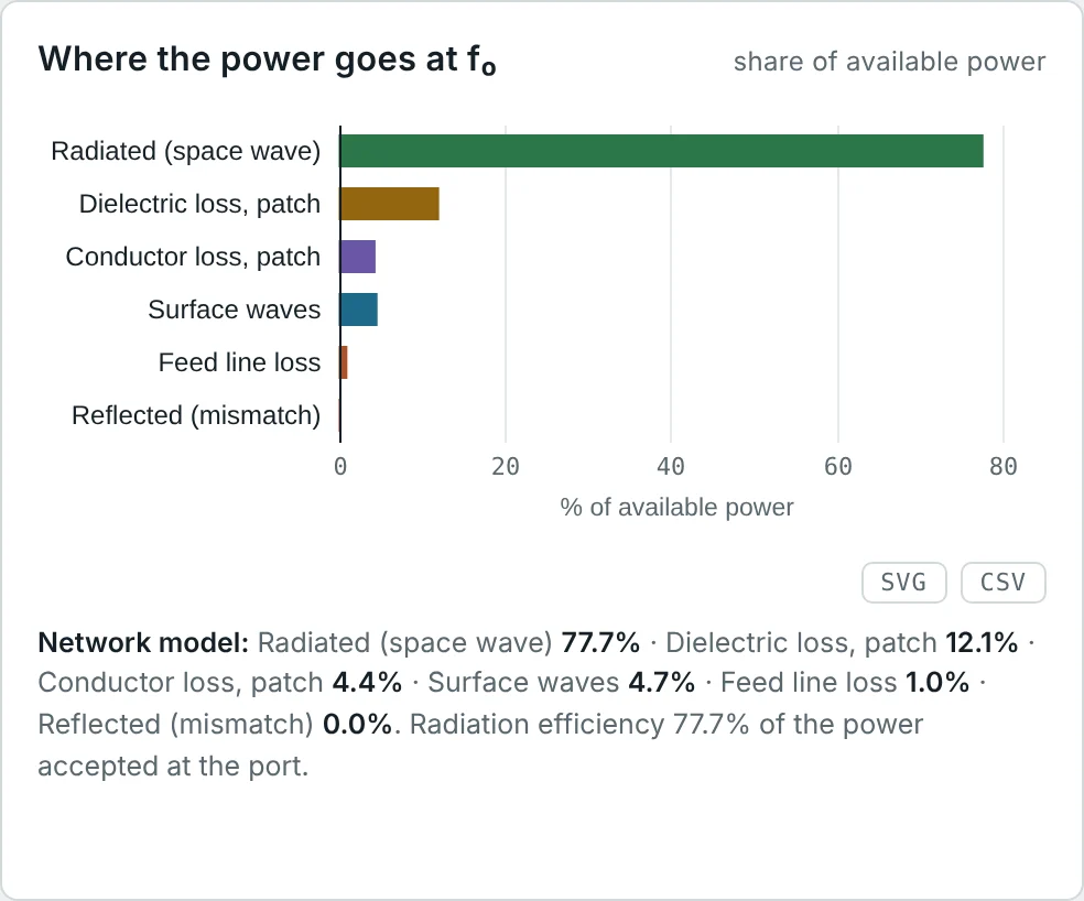
A patch on a grounded substrate also launches surface waves that travel along the dielectric slab instead of radiating. They are not dissipated, but they carry power away from the main beam, diffract at the board edges into unwanted directions (raising the back lobe and cross-polarization) and couple to neighbouring elements. The space-wave efficiency e_sw falls as the substrate becomes thicker or its permittivity higher; for thin substrates (h/λ₀ ≲ 0.02) it stays above about 90%. The calculator's circularly polarized RO4003C patch (h = 1.524 mm, ε_r = 3.55 at 2.45 GHz) has e_sw = 91.6%.

Practical Methods to Improve Antenna Efficiency

Make the antenna as large as allowed. Use the full available volume; fold or meander rather than shrink.
Use good conductors with enough cross-section: wide strips, thick wires, copper or silver plating, smooth foil at high frequencies.
Choose a low-loss substrate (tan δ ≤ 0.004) for printed antennas above about 1 GHz, or use an air-spaced patch.
Use high-Q tuning components: air-wound coils, vacuum or ceramic C0G capacitors, and as few matching components as possible.
Improve the ground: 16–120 radials under a monopole, or an elevated ground plane.
Keep lossy materials out of the reactive near field: clearance from batteries, displays, plastic housings and the body.
Prevent common-mode current on the feed cable with a balun or choke, so the cable does not become a lossy part of the antenna.

Measuring Antenna Efficiency

The Wheeler cap method encloses a small antenna in a conducting shell that stops it radiating without disturbing its near field. Inside the cap, R_r disappears from the input resistance but R_L remains. For an antenna that behaves as a series RLC near resonance:

Wheeler-cap efficiency (series-resonant antenna)

R_{fs} = R_{r} + R_{L} R_{cap} = R_{L} e_{cd} = \frac{R_{fs} - R_{cap}}{R_{fs}}

The cap must be larger than the reactive near field (radius ≳ λ/2π) but small enough not to resonate itself. Parallel-resonant antennas use conductances instead of resistances.

Other methods: integrating a full 3D gain pattern (P_rad from the pattern, P_in from the source and S₁₁); reverberation chambers, which compare the antenna with a reference of known efficiency in a statistically uniform field; and radiometric methods that measure the noise temperature (Example 8).

Worked Examples

Total Efficiency of the VHF Dipole

Problem: The 146 MHz copper dipole has e_cd = 99.7% and |Γ| = 0.180 on 50 Ω. Find e_r and e₀ in percent and dB.

e_{r} = 1 - {0.180}^{2} = 0.968 e_{0} = 0.968 \times 0.997 = 0.965 (- 0.16 dB)

Answer: e_r = 96.8%, e₀ = 96.5% (−0.16 dB)

Directivity 2.14 dBi − 0.16 dB = 1.98 dBi: exactly the realized gain the calculator reports. A full-size wire antenna is limited by its match, not its losses.

FR-4 vs Rogers: What Efficiency Costs in Gain

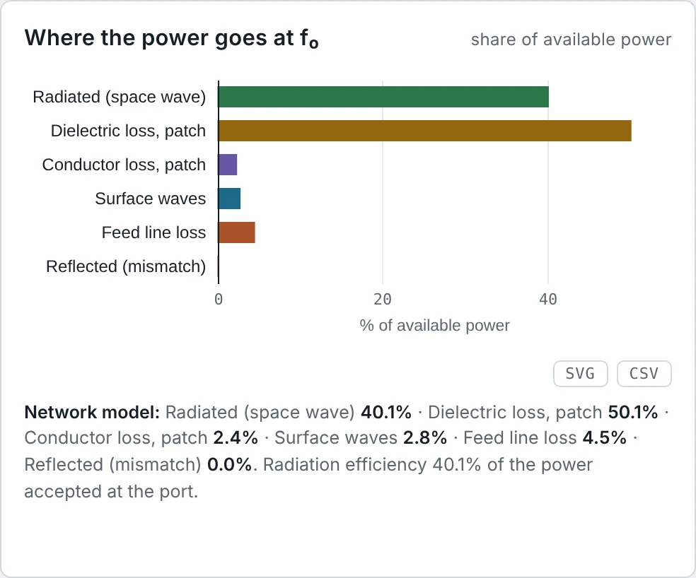
Problem: The FR-4 patch has D = 6.45 dBi and e_cd = 40.1%; the Rogers patch D = 6.72 dBi and e_cd = 77.7%. Find each gain and the difference.

G_{FR4} = 6.45 + 10 \log 0.401 = 6.45 - 3.97 = 2.48 dBi G_{RO} = 6.72 - 1.10 = 5.62 dBi

Answer: 2.48 dBi vs 5.62 dBi — the low-loss substrate gains 3.1 dB

3 dB is the difference between needing two base stations and one. For a 2.45 GHz product the extra substrate cost is usually the cheapest way to buy it.

Breaking Down Patch Losses with Q

Problem: The FR-4 patch has unloaded Q₀ = 27.6 and e_cd = 40.1%; FR-4 has tan δ = 0.02. Find Q_rad and the Q of the remaining losses (conductor plus surface wave).

Q_{rad} = \frac{Q_{0}}{e_{cd}} = \frac{27.6}{0.401} = 68.8 \frac{1}{Q_{other}} = \frac{1}{27.6} - \frac{1}{68.8} - 0.02 = 0.0017

Answer: Q_rad ≈ 69, Q_d = 50, Q_other ≈ 590

Dielectric loss (1/Q_d = 0.020) is 55% of the total loss rate 1/Q₀ = 0.036, matching the 50% dielectric loss in the calculator's power budget. Copper loss is minor; the substrate is the problem.

How Much Does Coil Q Matter?

Problem: The 1 m dipole at 30 MHz from Part 7 has R_r = 1.97 Ω and X_A = −1926 Ω. Find the efficiency with a loading coil of Q = 200 and Q = 500 (neglect wire loss).

R_{coil} = \frac{1926}{200} = 9.63 Ω \Rightarrow e_{cd} = \frac{1.97}{11.6} = 17 % R_{coil} = 3.85 Ω \Rightarrow e_{cd} = 34 %

Answer: 17% (−7.7 dB) with Q = 200; 34% (−4.7 dB) with Q = 500

Improving the coil is worth 3 dB. Doubling the antenna length to 0.2 λ would do far more (Fig 2): R_r rises fourfold and the reactance falls by more than half.

Ground Loss Under a Monopole

Problem: A quarter-wave broadcast monopole has R_r = 36 Ω. With 4 short radials the ground-loss resistance is 10 Ω; with 120 quarter-wave radials it is 2 Ω. Compare the radiation efficiencies.

e_{4} = \frac{36}{46} = 78 % (- 1.07 dB) e_{120} = \frac{36}{38} = 95 % (- 0.23 dB)

Answer: 78% vs 95% — 0.84 dB, equivalent to raising a 50 kW transmitter to 61 kW

The ground currents return to the base of the monopole through the soil; radials give them a low-resistance path. The FCC standard for AM stations is 120 radials of λ/4.

Dielectric Q of Common Substrates

Problem: A patch on a substrate radiates with Q_rad = 60 and has negligible conductor loss. Find e_cd for FR-4 (tan δ = 0.02), RO4350B (0.0037) and PTFE (0.0009).

e_{cd} = \frac{1 / Q_{rad}}{1 / Q_{rad} + \tan δ} : \frac{0.0167}{0.0367} = 45 %, \frac{0.0167}{0.0204} = 82 %, \frac{0.0167}{0.0176} = 95 %

Answer: 45% (FR-4), 82% (RO4350B), 95% (PTFE)

The rule of thumb for a patch: e_cd ≈ 1/(1 + Q_rad tan δ). Efficiency suffers whenever Q_rad·tan δ approaches 1.

Wheeler-Cap Measurement

Problem: A small series-resonant antenna measures R = 52 Ω in free space and R = 6 Ω inside a Wheeler cap. Find its radiation efficiency.

e_{cd} = \frac{52 - 6}{52} = 0.885 = - 0.53 dB

Answer: 88.5%

R_r = 46 Ω and R_L = 6 Ω. The method needs no anechoic chamber — just a metal can and a network analyzer.

Why Efficiency Matters for Receiving: Noise

Problem: A GNSS antenna looks at a 50 K sky. Its losses are at 290 K. With e_cd = 50% and a receiver noise temperature of 75 K, how much does the loss degrade the signal-to-noise ratio compared with a lossless antenna?

T_{A} = e_{cd} T_{sky} + (1 - e_{cd}) T_{phys} = 25 + 145 = 170 K

Δ SNR = 10 \log 0.5 - 10 \log \frac{170 + 75}{50 + 75} = - 3.0 - 2.9 = - 5.9 dB

Answer: about 5.9 dB worse — the signal falls 3 dB and the noise rises 2.9 dB

When the external noise is low (sky, satellites), a lossy antenna is doubly penalized. At HF, where atmospheric noise is thousands of kelvin, the same loss costs only the 3 dB on both signal and noise — almost nothing in SNR.

Total Radiated Power of a Phone

Problem: A phone delivers 23 dBm conducted power to an antenna with total efficiency 30% in talk position (hand and head). Find the TRP.

TRP = 23 + 10 \log 0.30 = 23 - 5.2 = 17.8 dBm

Answer: TRP = 17.8 dBm (60 mW of the 200 mW delivered)

Operators specify minimum TRP per band; antenna efficiency of 20–50% in use is typical below 1 GHz in smartphones, where the antenna is a small fraction of a wavelength and the hand is in its near field.

Stainless vs Copper on HF

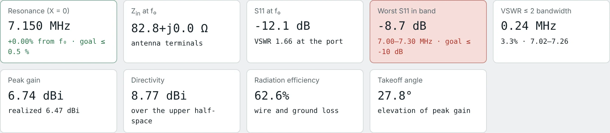
Problem: The calculator gives, for the 7.15 MHz dipole over average earth, radiation efficiency 62.6% (stainless) and 73.6% (copper), with the same directivity 8.77 dBi. Predict both gains and compare with the calculator values 6.74 and 7.44 dBi.

G_{ss} = 8.77 + 10 \log 0.626 = 6.74 dBi G_{cu} = 8.77 + 10 \log 0.736 = 7.44 dBi

Answer: 6.74 and 7.44 dBi, exactly as calculated — a 0.70 dB penalty for stainless steel

Both include about 22% ground loss, which only a higher antenna or better ground can reduce. On HF, ground loss usually costs more than conductor loss.

Summary

Total efficiency e₀ = e_r e_c e_d = (1 − |Γ|²) e_cd: mismatch, then conductor and dielectric loss.
Radiation efficiency e_cd = R_r/(R_r + R_L) = Q₀/Q_rad; it links gain and directivity, G = e_cd D.
Conductor loss is ½R_s∫|J_s|²dS with R_s = √(πfμ/σ); it concentrates where surface current is high.
Dielectric loss gives Q_d = 1/tan δ; on FR-4 it halves the efficiency of a patch, on low-loss substrates it is small.
Electrically small antennas are inefficient because R_r ∝ (L/λ)² while tuning losses grow; coil Q, ground systems and conductor size matter.
Mismatch efficiency can be fixed externally; radiation efficiency cannot. Efficiency is measured with Wheeler caps, pattern integration or reverberation chambers.
In receive mode, loss also adds thermal noise, which matters most when external noise is low.

Efficiency and match both depend on frequency. Part 10: Antenna Bandwidth and Quality Factor asks how wide a band an antenna can serve, and how the stored energy measured by Q limits it.

Put It Into Practice

Use the NEXT ANTENNAS calculators to apply the ideas from this article to real antennas.

Wire Antennas Dipole & Monopole Antenna Calculator Method of Moments design of dipoles, inverted-Vs and monopoles: length, impedance, S11, current, gain and 3D patterns. Open calculator → Antenna Design Patch Antenna Calculator Microstrip patch synthesis and simulation: dimensions, feed, S11, gain, efficiency and radiation patterns. Open calculator → Link & Power Link Budget Calculator Transmit power, antenna gains, path loss and margin for a complete wireless link. Open calculator → All Tools All RF Calculators Browse every NEXT ANTENNAS calculator for RF, microwave and antenna design. Open calculator →

Antenna Radiation Efficiency and Total Efficiency