Radiation Intensity and Power Density

Power density against distance for a 146 MHz station on log-log axes: a straight line falling at 20 dB per decade, crossing the public limit of 2 watts per square metre near 3 metres — Power density against distance in the main beam of a 146 MHz, 79 W EIRP station (RF Exposure Calculator). On log–log axes the inverse-square law is a straight line falling 20 dB per decade of distance. Try it in the RF Exposure Calculator →

Introduction to Radiated Power

An antenna fed with P_in watts radiates P_rad ≤ P_in (the rest is lost as heat, Part 9). That radiated power spreads over the sphere around the antenna, but not evenly: the radiation pattern of Part 4 shows its shape. To make the pattern quantitative we need two quantities:

Power density SWatts per square metre at a point in space. Depends on distance: it falls as 1/r² in the far field.

Radiation intensity UWatts per steradian in a direction. Independent of distance: U = r²S.

Total powerIntegrating either over a closed surface gives P_rad, the same for every sphere in the far field.

These are the ingredients of directivity and gain (Part 6), of the Friis equation (Part 13) and of every RF-exposure calculation.

The Poynting Vector

Electromagnetic fields carry energy. To see how much, and in which direction, start from Faraday's and Ampère–Maxwell's laws and apply the vector identity ∇·(E × H) = H·(∇ × E) − E·(∇ × H):

Poynting's theorem — derivation

\nabla \cdot (E \times H) = H \cdot (- μ \frac{\partial H}{\partial t}) - E \cdot (J + ε \frac{\partial E}{\partial t}) = - \frac{\partial}{\partial t} (\frac{1}{2} μ H^{2} + \frac{1}{2} ε E^{2}) - E \cdot J

∯_{A} S \cdot d A = - \frac{d}{d t} ∭_{V} (w_{e} + w_{m}) d V - ∭_{V} E \cdot J d V S = E \times H

Applying the divergence theorem to the first line gives an energy balance: power flowing out through the surface A equals the decrease of stored electric and magnetic energy inside, minus the power E·J delivered to currents (heat in a resistor, or −E·J > 0 for the source that drives an antenna). S = E × H, in W/m², is the Poynting vector.

The Poynting vector points in the direction of energy flow and its magnitude is the instantaneous power per unit area. For a plane wave in free space, E ⟂ H and |H| = |E|/η, so |S| = |E|²/η.

Average Power Density

Radio fields oscillate billions of times per second, so what matters is the time average over a period. With phasors, a real field is E(t) = Re{E e^(jωt)} = ½(E e^(jωt) + E* e^(−jωt)). Multiplying two such expressions:

Time-average Poynting vector — derivation

E (t) \times H (t) = \frac{1}{4} [E \times H^{*} + E^{*} \times H + E \times H e^{2 j ω t} + E^{*} \times H^{*} e^{- 2 j ω t}]

S_{av} = \frac{1}{T} \int_{0}^{T} E (t) \times H (t) d t = \frac{1}{2} Re {E \times H^{*}}

The terms at 2ω average to zero over a period. E and H are peak phasors here; with RMS phasors the ½ disappears. The imaginary part ½Im{E × H*} is the reactive power density — the stored energy that sloshes back and forth in the near field (Part 3).

In the far field, E and H are in phase, perpendicular, and |H| = |E|/η, so the average power density takes its simplest form:

Far-field power density

S_{av} = \frac{{| E |}^{2}}{2 η} = \frac{E_{rms}^{2}}{η} = η H_{rms}^{2} η \approx 377 Ω

This is the formula used by every field-strength meter that reports power density from a single E-field reading. It is valid only in the far field; in the reactive near field E and H must be measured separately.

Solid Angle and the Steradian

An angle in the plane is an arc length divided by radius, measured in radians; a full circle is 2π rad. A solid angle is the three-dimensional equivalent: an area on a sphere divided by the radius squared, measured in steradians (sr). A full sphere is 4πr²/r² = 4π sr.

Fig 1 — One steradian is the solid angle that cuts an area r² from a sphere of radius r. A small patch at angles (θ, φ) has area r² sin θ dθ dφ

Element of solid angle and the full sphere

d Ω = \frac{d A}{r^{2}} = \sin θ d θ d φ \int_{0}^{2 π} \int_{0}^{π} \sin θ d θ d φ = 2 π \times 2 = 4 π sr

The factor sin θ accounts for the shrinking circles of latitude near the poles. A full sphere contains 4π sr = 41 253 square degrees — the number that appears in the Kraus beamwidth formula of Part 6.

Radiation Intensity

The radiation intensity U in a given direction is the power radiated per unit solid angle. Because the far-field power density falls exactly as 1/r² while the area subtended by a fixed solid angle grows as r², their product is independent of distance:

Radiation intensity

U (θ, φ) = r^{2} S_{av} (r, θ, φ) = \frac{r^{2}}{2 η} [{| E_{θ} |}^{2} + {| E_{φ} |}^{2}] = \frac{1}{2 η} {| F (θ, φ) |}^{2}

Units: watts per steradian (W/sr). F(θ, φ) is the angular part of the far field, E = F e^(−jkr)/r (Part 2). U is a far-field quantity; its normalized form U/U_max is exactly the power pattern of Part 4.

Relationship between radiation intensity and power density

Quantity	Symbol	Units	Depends on r?	Use
Power density	S = ½Re{E × H*}	W/m²	Yes, ∝ 1/r²	Exposure, received power S·A_e
Radiation intensity	U = r²S	W/sr	No	Pattern, directivity, gain
Radiated power	P = ∯U dΩ	W	No	Efficiency, radiation resistance

Total Radiated Power

Adding up the power in every direction gives the total radiated power. In terms of power density over a sphere of radius r, or equivalently in terms of radiation intensity over the full solid angle:

Total radiated power

P_{rad} = ∯_{A} S_{av} \cdot d A = \int_{0}^{2 π} \int_{0}^{π} U (θ, φ) \sin θ d θ d φ

For a pattern that does not depend on φ (any antenna symmetric about the z-axis), the φ integral is simply 2π, leaving a single integral in θ.

Standard integrals

Many patterns can be written as, or approximated by, simple powers of sin θ or cos θ. Using the substitution x = cos θ (dx = −sin θ dθ), the integrals reduce to polynomials:

Radiation intensity U	∫ over the sphere	P_rad	Typical antenna
B₀ (constant)	2π · 2	4π B₀	Isotropic (reference only)
B₀ sin θ	2π · π/2	π² B₀	Field ∝ √sin θ (exercise pattern)
B₀ sin²θ	2π · 4/3	(8π/3) B₀	Short (Hertzian) dipole, small loop
B₀ sin³θ	2π · 3π/8	(3π²/4) B₀	Narrower omnidirectional
B₀ [cos(π/2·cos θ)/sin θ]²	2π · 1.2188	7.658 B₀	Half-wave dipole (needs Cin, Part 6)
B₀ cosⁿθ, 0 ≤ θ ≤ π/2	2π/(n + 1)	2π B₀/(n + 1)	Patch, horn, dish approximations

Fig 2 — Radiation intensity patterns with the same maximum (linear power scale, 0° at the top). Narrower patterns radiate less total power for the same peak — the idea behind directivity (Part 6)

sin θ: P = 9.87 B₀sin²θ: P = 8.38 B₀sin³θ: P = 7.40 B₀

cos⁴θ (upper half): P = 1.26 B₀

Radiation Intensity in Different Directions

Knowing U(θ, φ) and the distance, the power density in any direction follows immediately: S = U/r². In practice U is rarely given directly. Instead, antennas are described by their gain G(θ, φ) (Part 6), which compares U with the intensity of a lossless isotropic antenna fed with the same power:

Radiation intensity and power density from gain

U (θ, φ) = G (θ, φ) \frac{P_{in}}{4 π} S (r, θ, φ) = \frac{P_{in} G (θ, φ)}{4 π r^{2}}

This single line connects antenna theory to link budgets and RF exposure. In the direction of maximum gain the product P_in·G is the EIRP.

Isotropic Radiation and Power Distribution

An isotropic radiator radiates equally in all directions. It cannot be built — no real antenna can produce a transverse field that is uniform over a whole sphere (the "hairy ball" theorem forbids it) — but it is the universal reference. Its radiation intensity and power density are

Isotropic source

U_{0} = \frac{P_{rad}}{4 π} S_{0} = \frac{P_{rad}}{4 π r^{2}} E_{rms} = \sqrt{η S_{0}} = \frac{\sqrt{30 P_{rad}}}{r}

The last form uses η/4π = 120π/4π = 30 Ω. It gives the RMS field of any antenna in a given direction if P_rad is replaced by the EIRP in that direction.

EIRP and ERP

Regulators and link engineers describe a transmitter by its effective isotropic radiated power: the power that an isotropic antenna would need to produce the same power density in the direction of interest.

EIRP, ERP and field strength in practical units

EIRP = P_{t} G_{t} / L_{feed} ERP = \frac{EIRP}{1.64} E (dBµV/m) = EIRP (dBm) - 20 \log_{10} d_{km} + 44.77

ERP uses a half-wave dipole (G = 1.64, 2.15 dBi) as the reference instead of an isotropic antenna. The dB formula follows from E = √(30·EIRP)/r: for 1 mW at 1 km, E = 173 µV/m = 44.77 dBµV/m. Decibels are explained in our dB, dBm and dBi guide.

Power density exposure limits against frequency for FCC, ICNIRP 2020, ICNIRP 1998 and Safety Code 6, lowest between about 30 and 300 megahertz — Exposure limits on power density against frequency (RF Exposure Calculator). Limits are lowest between about 30 and 300 MHz, where the human body absorbs most efficiently, and rise above that range. Try it in the RF Exposure Calculator →

Beam Solid Angle

A useful way to summarize how concentrated a pattern is: imagine that all the power were radiated uniformly at the maximum intensity U_max, inside a cone, and nothing outside it. The solid angle of that cone is the beam solid angle Ω_A:

Beam solid angle

P_{rad} = U_{max} Ω_{A} \Rightarrow Ω_{A} = \int_{0}^{2 π} \int_{0}^{π} U_{n} (θ, φ) \sin θ d θ d φ U_{n} = \frac{U}{U_{max}}

Ω_A is the integral of the normalized power pattern. An isotropic source has Ω_A = 4π; a short dipole 8π/3 = 8.38 sr; a cos⁴θ beam 2π/5 = 1.26 sr. The ratio 4π/Ω_A is the directivity of Part 6.

Pattern	Ω_A (sr)	Fraction of the sphere	4π/Ω_A
Isotropic	12.57	100%	1.00
Short dipole (sin²θ)	8.38	67%	1.50
Half-wave dipole	7.66	61%	1.64
cos²θ, upper hemisphere	2.09	17%	6.0
cos⁴θ, upper hemisphere	1.26	10%	10.0
Pencil beam 10° × 10°	≈ 0.030	0.24%	≈ 410

Average Power for Pulsed and Modulated Signals

The Poynting average over one RF cycle gives the power density of the carrier. Real transmitters switch on and off (radar pulses, TDD frames, push-to-talk) or vary their envelope (AM, OFDM). Exposure limits and heating depend on the power averaged over seconds to minutes, while receivers and breakdown depend on the peak:

Duty cycle and time-averaged power density

P_{avg} = P_{peak} \cdot τ \cdot PRF = P_{peak} \cdot δ {\bar{S}}_{time} = δ \frac{P_{peak} G}{4 π r^{2}}

τ is the pulse width, PRF the pulse repetition frequency and δ the duty cycle. A radar with 1 MW peak, 1 µs pulses and 1 kHz PRF has δ = 0.001 and an average power of 1 kW. For rotating antennas the exposure is further reduced by the fraction of time the beam points at the observer.

Power Density from Several Sources

Power densities from independent transmitters on different frequencies add (their fields are uncorrelated, so the cross terms in |E₁ + E₂|² average to zero). Because the limits depend on frequency, compliance is judged by the sum of the fractions of each limit:

Total exposure ratio and field-strength conversion

TER = \sum_{i} \frac{S_{i}}{S_{lim, i}} \leq 1 S (dBm/m²) = E (dBµV/m) - 115.8

The second relation follows from S = E²/377: 10 log₁₀(377) = 25.8 dB, and the conversions µV → V (−120 dB) and W → mW (+30 dB) give −115.8 dB in total. It holds only in the far field.

The RF Exposure Calculator has a multi-source step that applies this rule to typical rooftop sites with cellular, 5G, microwave and broadcast transmitters.

Radiation Intensity Calculations: A Recipe

Get the far field. From a formula (Part 2), a simulator or a measurement, write E = F(θ, φ) e^(−jkr)/r.
Form U. U = |F|²/(2η) with peak phasors (or |F_rms|²/η).
Integrate. P_rad = ∫∫U sin θ dθ dφ, analytically for simple patterns, numerically otherwise (Example 6).
Normalize. U_max/U₀ = 4πU_max/P_rad is the directivity (Part 6); P_rad = ½|I|²R_r gives the radiation resistance (Part 7).
Scale to distance. S = U/r² in the far field; check that r is beyond the far-field distance (Part 3).

Worked Examples

Power Density of a Plane Wave

Problem: A far-field wave has a peak electric field of 10 V/m. Find the average power density and the peak magnetic field.

S_{av} = \frac{10^{2}}{2 \times 376.7} = 0.133 W/m² H = \frac{10}{376.7} = 26.5 mA/m

Answer: 0.133 W/m² (13.3 µW/cm²); H = 26.5 mA/m peak

The same field quoted as 10 V/m RMS would give twice the power density, 0.265 W/m². Always check whether a field value is peak or RMS — exposure standards use RMS.

Real and Reactive Power Density

Problem: In the near field of an antenna, a transverse E = 5∠0° V/m (peak) and the perpendicular H = 0.02∠−30° A/m. Find the real (time-average) and reactive power densities.

\frac{1}{2} E H^{*} = \frac{1}{2} (5) (0.02 ∠ + 30 °) = 0.05 ∠ 30 ° = 0.0433 + j 0.025

Answer: S_av = 43.3 mW/m² outward; 25 mvar/m² reactive

The ratio |E|/|H| = 250 Ω and the 30° phase difference both show that this point is not in the far field. Multiplying |E|²/(2η) instead would give 33.2 mW/m² — a 23% error.

From the Far Field to U and P_rad

Problem: An antenna's far field is E_θ = (10/r) sin θ e^(−jkr) V/m (peak), E_φ = 0. Find U(θ), P_rad and the ratio of the maximum to the average radiation intensity.

U = \frac{10^{2}}{2 \times 376.7} \sin^{2} θ = 0.1327 \sin^{2} θ W/sr P_{rad} = \frac{8 π}{3} (0.1327) = 1.112 W \frac{U_{max}}{U_{av}} = \frac{0.1327}{1.112 / 4 π} = 1.50

Answer: U = 0.133 sin²θ W/sr; P_rad = 1.11 W; U_max/U_av = 1.5

This is a short dipole. The ratio 1.5 is its directivity — Part 6 formalizes exactly this calculation.

Integrating U = B₀ sin θ

Problem: An antenna has U = B₀ sin θ with B₀ = 1 W/sr. Find P_rad.

P_{rad} = \int_{0}^{2 π} \int_{0}^{π} B_{0} \sin^{2} θ d θ d φ = 2 π B_{0} \cdot \frac{π}{2} = π^{2} B_{0} = 9.87 W

Answer: 9.87 W

Note the extra sin θ from dΩ: U = B₀ sin θ becomes sin²θ inside the integral. Forgetting the Jacobian sin θ is the most common error in radiated-power calculations.

A Directional cos⁴θ Antenna

Problem: A horn-like antenna has U = 2 cos⁴θ W/sr for 0 ≤ θ ≤ 90° and zero behind. Find P_rad and the power density 100 m away on axis.

P_{rad} = 2 π \cdot 2 \int_{0}^{1} x^{4} d x = \frac{4 π}{5} = 2.51 W S = \frac{U_{max}}{r^{2}} = \frac{2}{100^{2}} = 200 µW/m²

Answer: P_rad = 2.51 W; S = 200 µW/m² on axis at 100 m

An isotropic antenna radiating 2.51 W would give only 20 µW/m² at 100 m. The factor 10 = 2(n + 1) is the directivity of the cos⁴θ pattern.

Numerical Integration: Half-Wave Dipole

Problem: A half-wave dipole with I₀ = 1 A has U = (ηI₀²/8π²)[cos(π/2·cos θ)/sin θ]² = 4.775 F²(θ) W/sr. Estimate P_rad with the midpoint rule using 10° steps.

θ (midpoint)	5°	15°	25°	35°	45°	55°	65°	75°	85°
F² sin θ	0.0004	0.0111	0.0509	0.1369	0.2788	0.4706	0.6845	0.8734	0.9851

\int_{0}^{π} F^{2} \sin θ d θ \approx 2 \times 3.4917 \times \frac{π}{18} = 1.2188 P_{rad} = 2 π \times 4.775 \times 1.2188 = 36.57 W

Answer: P_rad ≈ 36.6 W — the midpoint rule with 18 points matches the exact Cin(2π)/2 = 1.2188 to four digits

Smooth patterns integrate very accurately with a coarse grid; patterns with many narrow side lobes need steps finer than the lobe width. The column sum, 3.4917, is doubled because the pattern is symmetric about 90°.

Field of an Isotropic Source

Problem: An isotropic source radiates 100 W. Find the power density and RMS field strength at 1 km.

S_{0} = \frac{100}{4 π {(1000)}^{2}} = 7.96 µW/m² E_{rms} = \frac{\sqrt{30 \times 100}}{1000} = 54.8 mV/m

Answer: 7.96 µW/m² and 54.8 mV/m (94.8 dBµV/m)

Check with the dB formula: EIRP = 50 dBm, d = 1 km → 50 − 0 + 44.77 = 94.77 dBµV/m.

Power Density Near a Wi-Fi Access Point

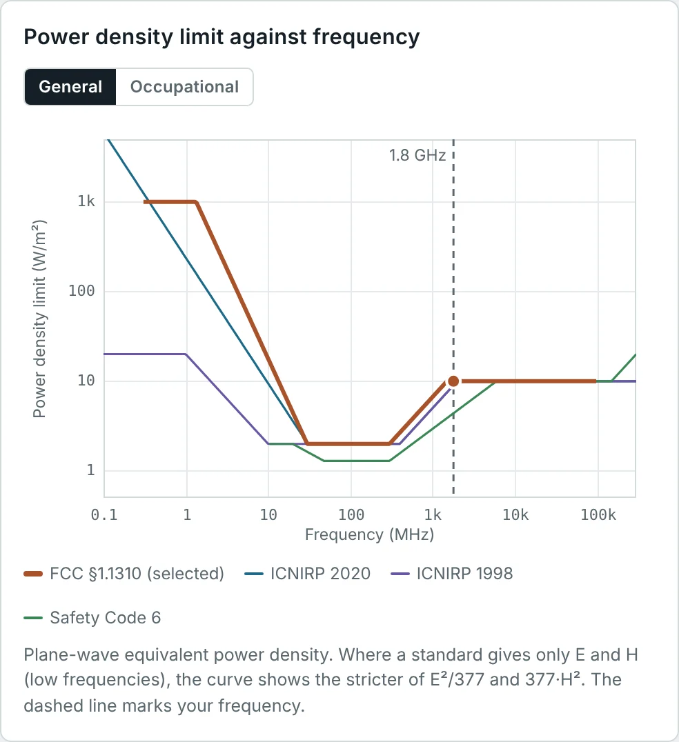
Problem: A 2.45 GHz access point transmits 100 mW into a 5 dBi antenna. Find the power density at 1 m and at 20 cm in the direction of maximum gain, and compare with the 10 W/m² FCC general-public limit.

EIRP = 0.1 \times 10^{0.5} = 0.316 W S (1 m) = \frac{0.316}{4 π} = 25 mW/m² S (0.2 m) = 0.63 W/m²

Answer: 25 mW/m² at 1 m and 0.63 W/m² at 20 cm — 0.25% and 6% of the limit

The 20 cm figure is the separation distance used for mobile-device RF evaluations under FCC rules. At 20 cm and 2.45 GHz (λ = 12 cm) the far-field formula is a reasonable, slightly conservative estimate.

Field Strength of an FM Station

Problem: An FM station has an ERP of 5 kW. Find the EIRP and the field strength in dBµV/m at 1 km and 30 km (free-space estimate).

EIRP = 1.64 \times 5000 = 8.2 kW = 69.1 dBm E_{1 km} = 69.1 + 44.8 = 113.9 dBµV/m E_{30 km} = 113.9 - 29.5 = 84.4 dBµV/m

Answer: 8.2 kW EIRP; 113.9 dBµV/m (0.50 V/m) at 1 km; 84.4 dBµV/m (17 mV/m) at 30 km

Real coverage predictions add terrain and ground-reflection losses (ITU-R P.1546), but the free-space value is the starting point and an upper bound for line-of-sight paths.

Exposure in Front of a Cellular Sector

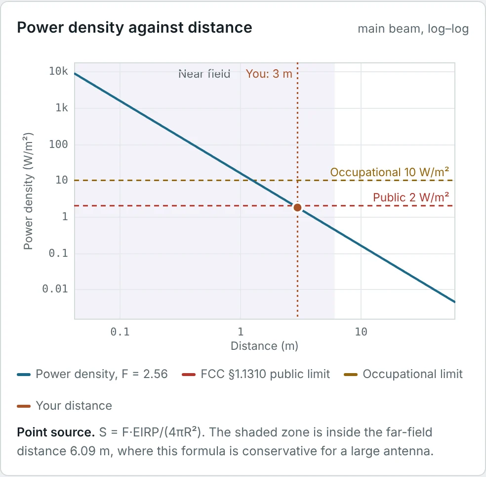
Problem: A sector antenna has an EIRP of 3.57 kW (2 × 40 W, 17.5 dBi, 1 dB feeder). Using the ground-reflection factor F = 2.56, find the power density and E-field 10 m away in the main beam.

S = \frac{2.56 \times 3570}{4 π \times 10^{2}} = 7.27 W/m² E_{rms} = \sqrt{7.27 \times 377} = 52.4 V/m

Answer: 7.27 W/m², 52.4 V/m — 73% of the FCC 10 W/m² public limit at 1.8 GHz

The RF Exposure Calculator reports 7.28 W/m² and 52.4 V/m for this case. F = 2.56 = (1 + 0.6)² allows for a ground reflection adding 60% to the field in phase.

Summary

Poynting's theorem, derived from Maxwell's curl equations, shows that S = E × H is the power flow per unit area.
For sinusoidal fields the average power density is S_av = ½Re{E × H*}; in the far field S_av = |E|²/(2η) = E_rms²/377.
Solid angle is measured in steradians, dΩ = sin θ dθ dφ, and a sphere has 4π sr.
Radiation intensity U = r²S_av (W/sr) is independent of distance and equals |F|²/(2η); normalized, it is the power pattern.
Total radiated power is P_rad = ∫∫U sin θ dθ dφ; simple patterns integrate in closed form, others numerically.
An isotropic source has U₀ = P/4π and S₀ = P/(4πr²); any antenna is described by its EIRP, with E_rms = √(30·EIRP)/r and E(dBµV/m) = EIRP(dBm) − 20 log d_km + 44.77.
The same formulas, with a reflection factor, are the basis of RF-exposure compliance distances.

Comparing U_max with the average intensity P_rad/4π gives a single number for how strongly an antenna concentrates its power. Part 6: Antenna Directivity and Gain defines it, derives it for the standard antennas, and adds losses to obtain gain.

Put It Into Practice

Use the NEXT ANTENNAS calculators to apply the ideas from this article to real antennas.

Link & Power RF Exposure & MPE Calculator Power density, field strength, near- and far-field regions and safe distances against FCC and ICNIRP limits. Open calculator → Link & Power Link Budget Calculator Transmit power, antenna gains, path loss and margin for a complete wireless link. Open calculator → Wire Antennas Dipole & Monopole Antenna Calculator Method of Moments design of dipoles, inverted-Vs and monopoles: length, impedance, S11, current, gain and 3D patterns. Open calculator → All Tools All RF Calculators Browse every NEXT ANTENNAS calculator for RF, microwave and antenna design. Open calculator →