The Central Question of Wireless Engineering
Every wireless system — a Wi-Fi router, a GPS receiver, a satellite downlink, a radar — must answer a single fundamental question before anything else: given a transmitter radiating some amount of power, how much of it arrives at the receiver? The answer to that question determines whether the link works at all, what data rate is achievable, how far the system can reach, and how much margin exists against interference and fading.
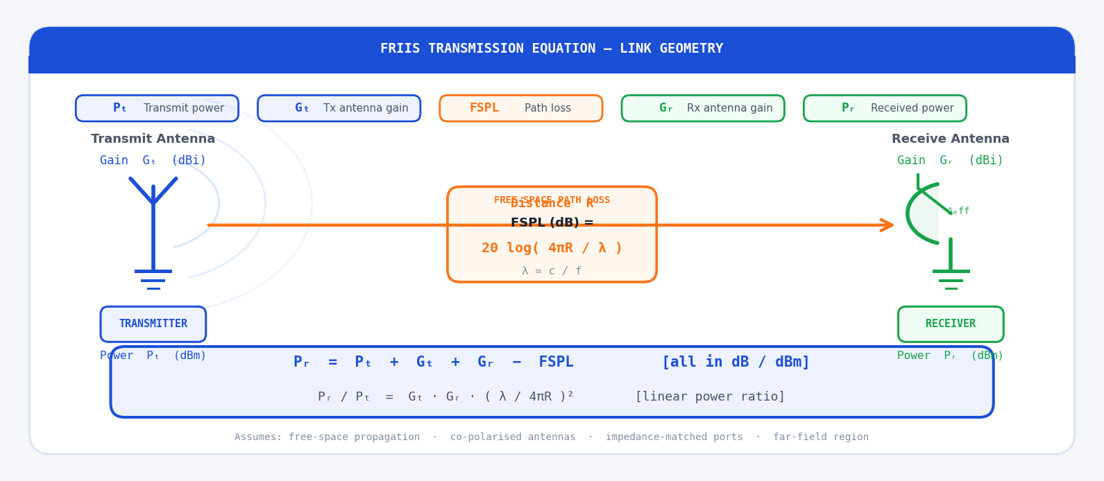
Harald T. Friis of Bell Labs derived the equation that answers this question in 1946. The Friis transmission equation relates the received power P_r to the transmitted power P_t through three factors: the gain of the transmit antenna G_t, the gain of the receive antenna G_r, and the free-space path loss that accounts for how a radio wave spreads as it propagates through space. Every link budget calculation in RF engineering is, at its core, an application of the Friis equation.
The Friis equation is derived for free-space propagation — no reflections, no atmospheric absorption, no obstructions, perfectly matched and co-polarised antennas. Real links deviate from these ideal conditions and require additional loss terms. But free space is the reference baseline from which all real-world propagation models begin, and understanding Friis exactly is a prerequisite for understanding those more complex models.
Deriving the Friis Equation from First Principles
Step 1 — Power Density from an Isotropic Radiator
Start with the simplest possible transmitter: an isotropic antenna — a hypothetical point source that radiates equally in all directions. If the transmitter delivers power P_t to this antenna, the power spreads uniformly over the surface of an expanding sphere. At distance R, the surface area of that sphere is 4πR², so the power density (power per unit area, in W/m²) is:
The transmit antenna radiates into a sphere of area 4πR². The effective aperture A_eff of the receive antenna intercepts a small portion of the total radiated power.
Step 2 — Adding Transmit Antenna Gain
A real transmit antenna is not isotropic — it concentrates power in preferred directions. The gain G_t of the transmit antenna (in the direction of the receiver) is defined as the ratio of the actual power density in that direction to what an isotropic radiator would produce with the same input power. The power density at distance R in the direction of the receiver therefore becomes:
Step 3 — Receive Antenna Effective Aperture
The receive antenna intercepts some of this incoming power density. How much it captures depends on its effective aperture A_eff (m²) — a measure of how large a cross-sectional area the antenna presents to the incoming wave. The power delivered to the receiver is:
Step 4 — Relating Effective Aperture to Receive Gain
Antenna theory shows that effective aperture and gain are related through wavelength λ. For any antenna, regardless of type or geometry:
Substituting this into the received power expression gives the Friis transmission equation:
A common misconception is that the λ² term means higher frequencies propagate worse in free space. This is wrong. The inverse square spreading (4πR²) is independent of frequency — a given power density at a given range is the same regardless of f. The λ² appears because the receive antenna's effective aperture shrinks with frequency at fixed gain. If you fix the physical aperture instead (e.g., the same dish antenna), received power is frequency-independent. The Friis equation is a statement about antenna gain, not about free-space propagation physics.
Free-Space Path Loss (FSPL)
It is conventional to separate the Friis equation into antenna terms and a propagation term. The free-space path loss FSPL is defined as the ratio of transmitted to received power between two ideal isotropic antennas (G_t = G_r = 1) at distance R:
Converting to decibels — by far the most practical form:
The most useful form in practice, with R in kilometres and f in GHz:
Every decade of distance adds 20 dB. Every doubling of frequency adds 6 dB. The lines are parallel — frequency shifts the curve vertically, distance determines the slope.
The Friis Equation in Decibels
Converting the Friis equation entirely to decibels transforms the multiplications and divisions into additions and subtractions — making link budget calculations straightforward arithmetic:
Real link budgets add further loss and gain terms — cable losses L_cable, connector losses, polarisation mismatch loss L_pol, atmospheric absorption L_atm, and receive system noise figure NF — extending the equation to:
Key Terms and Quantities
Effective Isotropic Radiated Power (EIRP)
EIRP is the product of the transmitted power and the transmit antenna gain, expressed in dBm or dBW. It represents the power that would need to be fed to an isotropic antenna to produce the same field strength in the direction of maximum gain:
Polarisation Mismatch Loss
The Friis equation assumes the transmit and receive antennas are co-polarised — the electric field orientations are aligned. When they are not, a polarisation mismatch loss L_pol must be included:
Impedance Mismatch Loss
Friis also assumes both antennas are perfectly impedance-matched to their connected transmission lines. Any mismatch causes a fraction of the available power to be reflected rather than radiated or received. The mismatch loss in terms of the reflection coefficient Γ at each antenna port is:
Receive Sensitivity and Link Margin
The received power P_r is only useful if it exceeds the receiver's minimum detectable signal (MDS), also called the receive sensitivity P_min. The link margin is the decibel cushion above this threshold:
Receive sensitivity is set by the thermal noise floor kTB (where k is Boltzmann's constant, T is noise temperature in kelvin, and B is the receiver bandwidth in Hz), raised by the receiver's noise figure NF. At room temperature (T = 290 K) the thermal noise floor is −174 dBm/Hz, so for a 20 MHz bandwidth receiver with NF = 7 dB: P_min = −174 + 10 log(20×10⁶) + 7 = −174 + 73 + 7 = −94 dBm. This is why low noise figures, narrow bandwidths, and high antenna gains are so important for long-range links.
The Complete Friis Equation
Including all mismatch and polarisation terms, the complete generalised Friis equation is:
In most practical link budgets these factors are handled separately as individual loss terms in the dB budget, which is cleaner and easier to audit. The key insight is that each imperfection — mismatch, polarisation misalignment, pointing error — is an independent multiplicative factor ≤ 1 in the power ratio, or equivalently a positive dB loss subtracted from the Friis baseline.
Questions & Worked Examples
Apply the Friis equation and link budget method to real-world RF systems. Work through each problem fully before reading the solution.
Wi-Fi Link Budget at 2.4 GHz
Problem: A Wi-Fi access point transmits +20 dBm through a 1 dB cable loss to a 3 dBi omni antenna. The client device is 30 m away with a 2 dBi antenna, 0.5 dB cable loss, and a receiver sensitivity of −80 dBm. Calculate: (a) FSPL at 2.4 GHz over 30 m, (b) received power P_r, (c) link margin.
33.9 dB of margin at 30 m is excellent — this link has room for significant multipath fading, obstructions, and body-loss effects without failing. At the sensitivity threshold of −80 dBm, this system could theoretically close the link at a maximum free-space distance where FSPL = 20 + 3 + 2 − 0.5 − 1 + 80 = 103.5 dB, which corresponds to R = 10^((103.5 − 92.44 − 7.6)/20) km = 10^(0.173) ≈ 1.49 km. Real indoor range is much shorter due to walls and multipath.
GPS Satellite Downlink
Problem: A GPS satellite transmits on L1 (1.575 GHz) with P_t = +13 dBW, transmit antenna gain G_t = +13 dBi, at a slant range of R = 22,200 km to a receiver with a patch antenna G_r = +3 dBi. Calculate the received power P_r in dBW and dBm.
−124.3 dBm is an extraordinarily weak signal — roughly 25 billion times below the thermal noise floor referenced to 1 mW. GPS receivers recover this signal using spread-spectrum (DSSS) processing gain and correlation, which provides typically 43 dB of processing gain. The effective received power after despreading is approximately −124.3 + 43 = −81.3 dBm — well above the receiver noise floor of around −130 dBm in a 50 Hz tracking bandwidth. This is one of the most impressive feats in consumer electronics engineering.
Maximum Range from Link Margin
Problem: A 915 MHz ISM-band sensor node transmits +27 dBm with a 0 dBi antenna. A gateway receiver at distance R has a 6 dBi directional antenna and sensitivity of −110 dBm. Cable and connector losses total 1.5 dB on each end. Ignoring other losses, find the maximum free-space range R_max.
261 km is an impressive free-space range — achievable in principle from a high tower or UAV to another elevated point with line-of-sight. The Earth's curvature limits ground-level line-of-sight to around 10–40 km depending on antenna heights. Real LoRaWAN and 915 MHz ISM deployments achieve 15–50 km in rural areas with elevated gateways — consistent with this calculation once terrain, ground reflections, and a realistic fade margin of 20–30 dB are accounted for.
Effect of Frequency on a Fixed Physical Link
Problem: Two identical horn antennas with a physical aperture of 0.01 m² each are used in a fixed 500 m microwave link. The transmitter outputs +30 dBm. Compare the received power at (a) 10 GHz and (b) 24 GHz, and explain the result physically.
For a horn antenna with physical aperture A, the aperture efficiency η ≈ 0.6, so A_eff = 0.6 × 0.01 = 0.006 m². Gain G = 4πA_eff/λ².
Received power is 7.6 dB higher at 24 GHz than at 10 GHz for the same physical aperture antennas. This confirms that the "frequency penalty" in the Friis λ² term is entirely an antenna gain effect. When the physical aperture is fixed, higher frequency gives higher gain, and that gain increase (2 × 7.6 = 15.2 dB more gain across both antennas) more than offsets the FSPL increase (7.6 dB more loss). This is why millimetre-wave 5G and fixed microwave backhaul links use compact high-gain dishes to achieve outstanding performance at 24, 28, and 60 GHz.
Link Closure with Polarisation and Impedance Mismatch
Problem: A 5.8 GHz FPV drone link transmits +27 dBm with a 3 dBi circular polarisation (CP) antenna. The ground receiver has a 5 dBi linear polarisation (LP) antenna with a measured VSWR of 1.8:1 (|Γ| = 0.286), and sensitivity of −85 dBm. The link distance is 1.5 km. Calculate: (a) polarisation mismatch loss between CP and LP, (b) impedance mismatch loss at receiver, (c) received power, (d) link margin.
Only 5.4 dB of margin at 1.5 km — this link is marginal. The dominant loss culprit is the 3 dB polarisation mismatch between the CP transmit and LP receive antennas. Replacing the ground receiver antenna with a CP antenna (matched polarisation) would immediately recover 3 dB, increasing the margin to 8.4 dB and the reliable range by approximately 40%. For FPV applications where reliable video link is safety-critical, a minimum margin of 10 dB and matched CP antennas on both ends are strongly recommended.