Introduction to Antenna Impedance Matching
Part 7 showed that an antenna presents an impedance Z_A = R_A + jX_A that depends on its geometry and frequency. Transmitters, receivers and cables are designed for a fixed reference impedance Z₀ — almost always 50 Ω (75 Ω in TV and cable systems). When Z_A ≠ Z₀, a fraction of the incident power is reflected at the antenna terminals. This article quantifies that fraction with four interchangeable numbers — reflection coefficient, return loss, VSWR and mismatch loss — and shows how to read them on a measured S₁₁ plot.
The transmission-line theory behind these quantities is developed in our Smith Chart & Impedance Matching series. Here we apply it to antennas, where the load is frequency-dependent, sits at the end of a lossy cable and may be balanced while the cable is not.
What Is Impedance Mismatch?
A transmission line forces a fixed ratio V/I = Z₀ on every wave travelling along it. At the antenna terminals, the total voltage and current must satisfy V/I = Z_A instead. If Z_A ≠ Z₀, a single forward wave cannot satisfy both conditions, so a second wave — the reflected wave — is created with exactly the amplitude and phase needed to make the totals fit. Mismatch is not a loss mechanism inside the antenna; it is the line and the antenna disagreeing about how much current a given voltage should drive.
Incident and Reflected Waves
On a lossless line with the antenna at z = 0 and the source at negative z, the voltage and current are sums of a forward wave and a reflected wave:
Reflection Coefficient
At the antenna (z = 0), V(0)/I(0) must equal Z_A:
Magnitude and phase of Γ
The magnitude |Γ| tells how much is reflected: |Γ|² is the fraction of incident power. The phase ∠Γ tells where the antenna sits on the Smith chart: positive phases (upper half) mean an inductive antenna, typically too long; negative phases (lower half) mean capacitive, typically too short; ∠Γ = 0° means purely resistive with R_A > Z₀, ∠Γ = 180° purely resistive with R_A < Z₀. The magnitude determines how bad a mismatch is; the phase determines how to fix it.
Moving a distance ℓ back along a lossless line toward the source rotates the phase of Γ but leaves its magnitude unchanged:
VSWR and Standing Waves
The forward and reflected waves interfere and create a standing-wave pattern along the line. The voltage magnitude oscillates between a maximum, where the two waves add in phase, and a minimum, where they oppose:
VSWR is the number traditionally read on an SWR meter and quoted on antenna datasheets ("VSWR ≤ 1.5:1 across the band"). Its maxima matter physically: the peak voltage on a 1 kW line with VSWR 3 is 1.5 times the matched value, which sets connector and capacitor ratings.
Return Loss
Return loss is the ratio of incident to reflected power in decibels — how far below the incident wave the reflection is:
Converting between the four measures
| Return loss | |Γ| | VSWR | Reflected power | Mismatch loss | Typical meaning |
|---|---|---|---|---|---|
| 3 dB | 0.708 | 5.85 | 50.1% | 3.02 dB | Badly mismatched |
| 6 dB | 0.501 | 3.01 | 25.1% | 1.26 dB | Acceptable for some phone bands at band edges |
| 9.54 dB | 0.333 | 2.00 | 11.1% | 0.51 dB | "VSWR 2:1" — common transmitter and antenna limit |
| 10 dB | 0.316 | 1.92 | 10.0% | 0.46 dB | The usual impedance-bandwidth criterion |
| 15 dB | 0.178 | 1.43 | 3.2% | 0.14 dB | Good match |
| 20 dB | 0.100 | 1.22 | 1.0% | 0.04 dB | Very good: base-station panel specification |
| 30 dB | 0.032 | 1.07 | 0.1% | 0.004 dB | Laboratory-grade load |
Reflected Power and Accepted Power
The time-average power carried by each wave on a line of real Z₀ is |V|²/(2Z₀). Because the forward and reflected waves are orthogonal travelling waves, their powers simply subtract:
This is the form used when the source is a matched Z₀ generator, which is the definition of S₁₁ and the normal situation for a transmitter with a 50 Ω output or a VNA. For an arbitrary complex source impedance Z_S, the general power-transfer factor is 4R_S R_A/|Z_S + Z_A|², which reaches 1 at the conjugate match Z_A = Z_S*. With Z_S = Z₀ real, it reduces to 1 − |Γ|².
The S₁₁ Parameter of an Antenna
In scattering-parameter language, an antenna is a one-port network (or a two-port, if the radiation is counted as a second port). S₁₁ is the ratio of the reflected to the incident wave at its port, with the port terminated in Z₀ — that is, S₁₁ = Γ referred to the measurement plane. A VNA displays it in several formats:
| VNA format | What is plotted | Best for |
|---|---|---|
| Log magnitude | 20 log₁₀|S₁₁| (dB) vs frequency | Resonance, bandwidth, datasheet plots |
| SWR | (1 + |S₁₁|)/(1 − |S₁₁|) | Transmitter compatibility, amateur radio practice |
| Smith chart | S₁₁ in the complex plane, with impedance grid | Diagnosing the mismatch and designing the match |
| Phase | ∠S₁₁ vs frequency | Electrical delay and cable length checks |
| Time domain | Inverse FFT of S₁₁ | Locating faults and reflections along a feeder |
On a multi-element array, each element also has mutual coupling terms S_ij. The active reflection coefficient of element i, Γ_i = Σ S_ij a_j/a_i, depends on the excitation of all the other elements and changes as the beam is steered — a phased array can be well matched at broadside and badly mismatched at a scan angle.
Interpreting S₁₁ Measurements
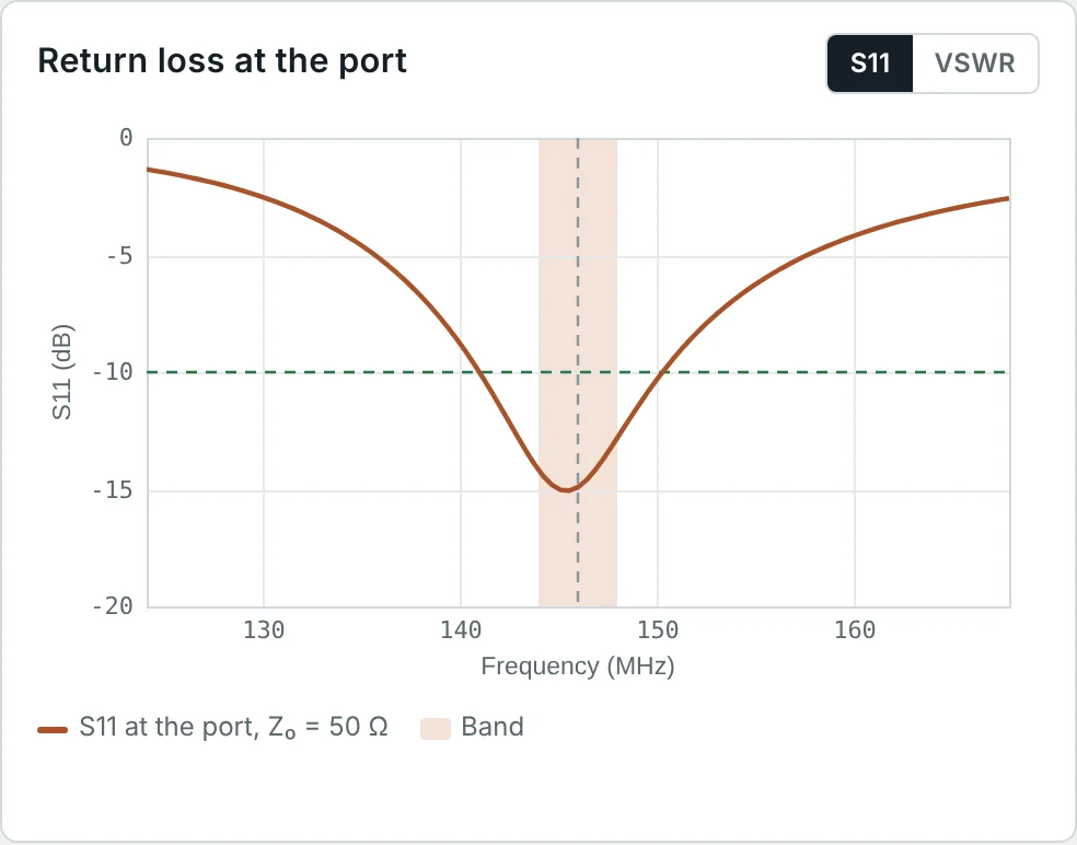
The S₁₁ plots of three calculator designs show the main features to look for:
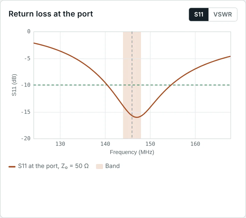
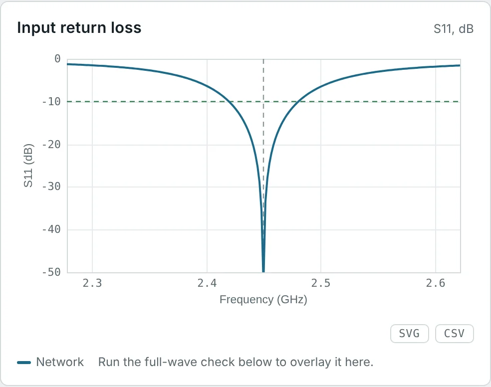
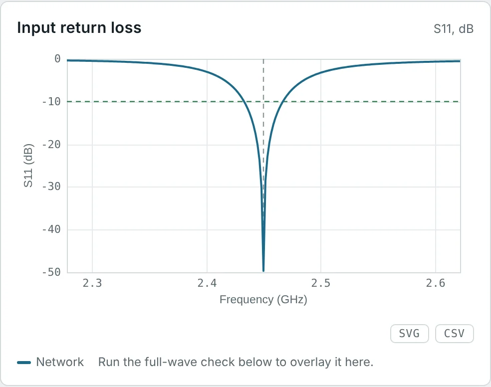
- Frequency of the minimum. Close to (but not always exactly at) the resonance; a dip below the design frequency means the antenna is too long, above means too short.
- Depth of the minimum. Shows how close R_A is to Z₀ at resonance. A very deep dip (−30 dB or better) only says the match is excellent at one frequency, not that the antenna is efficient.
- Width of the dip. The −10 dB (or VSWR 2) width is the impedance bandwidth of Part 10; a wider dip means lower Q.
- Several dips. Multi-band antennas, higher-order modes, or — if unexpected — a resonance in the cable shield or a nearby object.
- A suspiciously good, flat S₁₁. Usually loss, not good design: a lossy antenna, or a long lossy cable, absorbs power instead of reflecting it (Example 5). Low S₁₁ says power is accepted; Part 9 asks whether it is radiated.
How the Feed Cable Changes What You Measure
Always measure at the antenna end, or de-embed the cable. A transmitter's SWR meter at the bottom of a long, lossy feeder reports a reassuringly low VSWR even when the antenna is broken.
Methods to Improve Antenna Matching
| Method | How it works | Bandwidth | Typical use |
|---|---|---|---|
| Trim the antenna | Adjust length to move resonance (X = 0) to the design frequency | Native | Dipoles, monopoles, patches |
| Adjust the feed point | Inset feed (patch), off-centre feed, gamma or T match (Yagi): picks a point where R = Z₀ | Native | Patches, Yagis, OCF dipoles |
| L-network | One series and one shunt reactance; two solutions for any load | Narrow (set by the network Q) | PCB antennas, HF tuners |
| Quarter-wave transformer | A λ/4 line of Z_T = √(Z₀R_A) matches a resistive load | Moderate | Arrays, dipoles, patches |
| Stub matching | Short- or open-circuited line sections as reactances | Narrow | Microwave, waveguide |
| Balun / transformer | Converts balanced to unbalanced and often transforms impedance (1:1, 4:1, 9:1) | Broad | Dipoles, folded dipoles, end-fed wires |
| Multi-section / tapered transformers | Gradual impedance change | Broad | Wideband feeds |
Network design in detail, with Smith-chart constructions, is the subject of Impedance Matching Using the Smith Chart and our impedance-matching guide. For a resistive antenna R_A below Z₀, the L-network values follow from a single parameter, the network Q:
Worked Examples
A Resonant Dipole on 50 Ω
Problem: The 146 MHz calculator dipole has Z_A = 71.9 Ω at resonance. Find Γ, return loss, VSWR and mismatch loss on 50 Ω coax.
Exactly the calculator's S₁₁ = −14.9 dB and VSWR 1.44. The calculator's realized gain (1.98 dBi) is 0.14 dB below its gain (2.12 dBi): the mismatch loss.
An Exact Half-Wave Dipole on 75 Ω
Problem: A dipole cut to exactly λ/2 (Z_A = 73.1 + j42.5 Ω) is fed with 75 Ω cable. Find Γ in magnitude and phase, and the VSWR. What does the phase say?
The resistance is almost perfect for 75 Ω; the whole mismatch is the +j42.5 Ω reactance, shown by the large positive phase (upper Smith chart). Shortening the dipole by about 4% removes it.
Power Accounting at 10 dB Return Loss
Problem: 100 W is incident on an antenna with 10 dB return loss. Find the reflected and accepted power and the mismatch loss.
This is why −10 dB is the standard bandwidth criterion: 90% of the power is delivered, a loss most link budgets barely notice.
Reading a Forward/Reflected Power Meter
Problem: A directional wattmeter at the antenna reads 100 W forward and 11 W reflected. Find |Γ|, VSWR and the power delivered to the antenna.
Power meters measure the two waves separately, so their difference is always the delivered power, whatever the line length.
A Lossy Cable Hides a Poor Antenna
Problem: An antenna with VSWR 3 is fed through 30 m of cable with 3 dB loss. What VSWR does the transmitter see? What would an open circuit look like behind 5 dB of cable?
The cable absorbs 50% of the forward power and 50% of the reflection. A "good" SWR reading at the shack can coexist with a broken antenna — measure at the antenna.
Phase Rotation Along the Feed Line
Problem: At the antenna, Γ_A = 0.3∠−40°. What is Γ seen 0.1 λ_g back along a lossless line, and what impedance does that represent in a 50 Ω system?
The impedance changes with cable length but |Γ|, VSWR and return loss do not (on a lossless line). That is why matching must be designed at a specific reference plane.
L-Network Match for a Monopole
Problem: Match the 146 MHz monopole (Z_A = 35.9 Ω) to 50 Ω with a series inductor and shunt capacitor.
Check: 1/(35.9 + j22.5) = 0.0200 − j0.0125 S. The conductance is exactly 1/50 and the susceptance is cancelled by +j0.0125 S from the capacitor. In practice, drooping the radials of a ground-plane antenna does the same job mechanically.
Quarter-Wave Transformer for a Dipole
Problem: Match the 71.9 Ω dipole to 50 Ω with a quarter-wave transformer. What characteristic impedance and length (velocity factor 0.66) are needed at 146 MHz?
60 Ω coax is not standard; a common alternative is two parallel 120 Ω lines, or a 75 Ω section with a small residual mismatch. A quarter-wave of 75 Ω would transform 71.9 Ω to 78.2 Ω — worse — which illustrates that Z_T must lie between the two impedances.
Reading Bandwidth from S₁₁ Plots
Problem: From the calculator results: the dipole's VSWR ≤ 2 band is 9.64 MHz at 146 MHz; the FR-4 patch's −10 dB band is 60.7 MHz and the Rogers patch's 33.9 MHz, both at 2.45 GHz. Express each as a fractional bandwidth.
The low-loss Rogers patch has the narrower match: loss resistance broadens S₁₁ curves. A wide S₁₁ bandwidth is not automatically a virtue — Part 10 separates the two effects.
Turning S₁₁ into Realized Gain
Problem: A patch has 5.63 dBi gain and S₁₁ = −8 dB at a band edge. Find the realized gain there.
(Assuming the gain itself is unchanged at the band edge.) Realized gain, defined in Part 6, is the number that belongs in a link budget, because it already includes the mismatch.
Summary
- An impedance mismatch creates a reflected wave; its ratio to the incident wave is Γ = (Z_A − Z₀)/(Z_A + Z₀), derived from V/I = Z_A at the terminals.
- |Γ| sets how much is reflected, ∠Γ shows whether the antenna is inductive or capacitive; a line rotates ∠Γ by 2βℓ and a lossy cable reduces |Γ| by twice its loss.
- Return loss = −20 log|Γ|; |S₁₁| in dB is its negative. VSWR = (1 + |Γ|)/(1 − |Γ|).
- Accepted power is (1 − |Γ|²) of the incident power; mismatch loss −10 log(1 − |Γ|²) is small: 0.46 dB at 10 dB return loss.
- S₁₁ plots show resonance (dip frequency), match quality (dip depth) and impedance bandwidth (dip width); suspiciously good S₁₁ often means loss.
- Matching uses trimming, feed-point choice, L-networks (Q_n = √(Z₀/R_A − 1)), quarter-wave transformers (Z_T = √(Z₀R_A)), stubs and baluns.
A perfect match guarantees that power enters the antenna, not that it is radiated. Part 9: Antenna Radiation Efficiency and Total Efficiency follows the accepted power through conductor and dielectric losses to the total efficiency.
Put It Into Practice
Use the NEXT ANTENNAS calculators to apply the ideas from this article to real antennas.