How Antennas Radiate Electromagnetic Waves

Fig 1 — Electric field lines of an oscillating short dipole (black, centre), computed from the exact solution. Close to the dipole the lines start and end on its charges; beyond about λ/2 they close on themselves and travel outward as free waves

Introduction to Electromagnetic Radiation

Electromagnetic radiation is energy that leaves a source as a self-sustaining wave of electric and magnetic fields and never returns. It is different from the stored energy around a capacitor or an inductor, which flows back and forth between the circuit and its fields every cycle. An antenna is a structure designed so that a large fraction of the energy delivered to it becomes radiation, and as little as possible stays stored nearby.

Part 1 showed that the radiated power of a short current element is P_rad = 40π²(L/λ)²I₀². Here we derive the fields themselves. They explain where the power goes (the pattern, Part 4), where the stored energy lives (the near field, Part 3), and why the input impedance of an antenna has a reactive part (Part 7).

Needs accelerationCharges at rest and charges in uniform motion do not radiate; oscillating charges always accelerate.

Needs timeFields travel at the speed of light, so the field at distance r reflects the current at the earlier time t − r/c.

Falls as 1/rRadiation fields fall as 1/r, so their power, ∝ 1/r², flows through every sphere undiminished.

Relationship Between Electric and Magnetic Fields

Maxwell's equations couple the two fields. Faraday's law says a changing magnetic field produces a circulating electric field; the Ampère–Maxwell law says a changing electric field (displacement current) or a conduction current produces a circulating magnetic field. In phasor form, with time dependence e^jωt:

Maxwell's curl equations in phasor form (source current J)

\nabla \times E = - j ω μ H \nabla \times H = J + j ω ε E

Each changing field is the source of the other. Once a wave has left the antenna it no longer needs J: the two curl equations keep regenerating each other. Our Maxwell's Equations series develops these equations from first principles.

In a travelling plane wave, E, H and the direction of travel are mutually perpendicular, E and H are in phase, and |E|/|H| = η = √(μ/ε). Close to an antenna none of this is true: E and H are out of phase, have components along the direction of travel, and their ratio depends on distance. The transition between the two regimes is the central result of this article.

Time-Varying Fields and Retardation

For a static charge, the electric field everywhere responds instantly to the charge's position. In reality, information about a change travels at c. When the charge moves at time t, an observer at distance r learns about it only at t + r/c. This delay — retardation — is what allows fields to separate from their sources.

Mathematically, it is convenient to work with the magnetic vector potential A, defined by μH = ∇ × A. Substituting into Maxwell's equations with the Lorenz gauge gives a wave equation driven by the current, whose solution is the retarded potential:

Vector potential: wave equation and its solution

\nabla^{2} A + k^{2} A = - μ J A (r) = \frac{μ}{4 π} ∭_{V} J (r') \frac{e^{- j k R}}{R} d V^{'}

R = |r − r′| is the distance from each source point to the observer, k = 2π/λ. The factor e^(−jkR) is the phase delay of retardation: the potential at the observer reflects the current a time R/c earlier. Each bit of current contributes a spherical wave; the antenna's field is their sum.

This single integral is the foundation of antenna analysis. Every pattern in this series — dipole, array, patch — is an evaluation of it for a particular current distribution J. Simulators such as the Method of Moments solver in our Dipole & Monopole Antenna Calculator first solve for J on the wire and then evaluate this integral.

Accelerating Charges and Electromagnetic Radiation

The simplest radiator is one charge q that briefly accelerates. J. J. Thomson's argument shows why it radiates. Before the acceleration the field lines are straight and radial from the charge's old position; long after, they are radial from the new position. Information about the change travels outward at c, so the two regions are joined by a thin shell in which the field lines are bent sideways. That kink carries a transverse electric field that moves outward. Its strength, obtained by the geometry of the kink, is

Radiation field of an accelerating charge

E_{rad} = \frac{q a \sin θ}{4 π ε_{0} c^{2} r} E_{static} = \frac{q}{4 π ε_{0} r^{2}}

θ is measured from the direction of acceleration. The radiation field falls as 1/r while the Coulomb field falls as 1/r², so at large distance only the radiation survives. It is zero along the line of acceleration and maximum perpendicular to it — the sin θ pattern of every short dipole.

Deriving the Larmor formula

The radiated power density is S = E_rad²/η₀ (instantaneous fields), with η₀ = 1/(ε₀c). Integrate it over a sphere of radius r, using dA = 2πr² sin θ dθ:

Total radiated power by integration

P = \int_{0}^{π} \frac{q^{2} a^{2} \sin^{2} θ}{16 π^{2} ε_{0} c^{3} r^{2}} 2 π r^{2} \sin θ d θ = \frac{q^{2} a^{2}}{8 π ε_{0} c^{3}} \underset{4 / 3}{\underset{⏟}{\int_{0}^{π} \sin^{3} θ d θ}} = \frac{q^{2} a^{2}}{6 π ε_{0} c^{3}}

The r² cancels: the same power crosses every sphere, which is the defining property of radiation. The integral ∫sin³θ dθ = 4/3 appears again in the directivity of the short dipole (Part 6).

In an antenna, electrons oscillate sinusoidally along the conductor, so they accelerate continuously and radiate continuously. Their individual speeds are tiny — millimetres per second — but there are around 10²³ free electrons per cubic centimetre of copper, and their accelerations add coherently because they all move in step.

Current Distribution in an Antenna

What an antenna radiates is determined entirely by the current flowing on it. On a thin centre-fed wire, the feed launches waves that travel to the open ends and reflect, so the current is a standing wave. The current must vanish at the free ends, and to a very good approximation the distribution is sinusoidal:

Sinusoidal current on a thin centre-fed dipole of total length L

I (z) = I_{m} \sin [k (\frac{L}{2} - | z |)] I_{feed} = I (0) = I_{m} \sin (\frac{k L}{2})

For L ≪ λ the sine is nearly linear and the current is triangular (short dipole). For L = λ/2 it is a half-cycle with its maximum at the feed. For L = λ the feed sits at a current minimum, so the input impedance is very high (Part 7).

Current magnitude along a half-wave dipole: a half sine wave, maximum at the feed and zero at both tips — Half-wave dipole at 146 MHz (Method of Moments): the current is a half-cycle of a sine, largest at the centre feed. Try it in the Dipole & Monopole Antenna Calculator →

Current magnitude along a quarter-wave monopole: maximum at the base and falling to zero at the tip — Quarter-wave monopole on a ground plane: a quarter-cycle, largest at the base feed. With its image below the ground, it forms the same current as the dipole. Try it in the Dipole & Monopole Antenna Calculator →

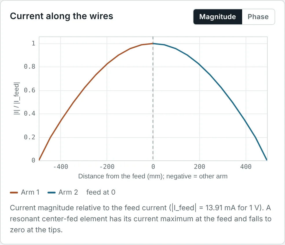
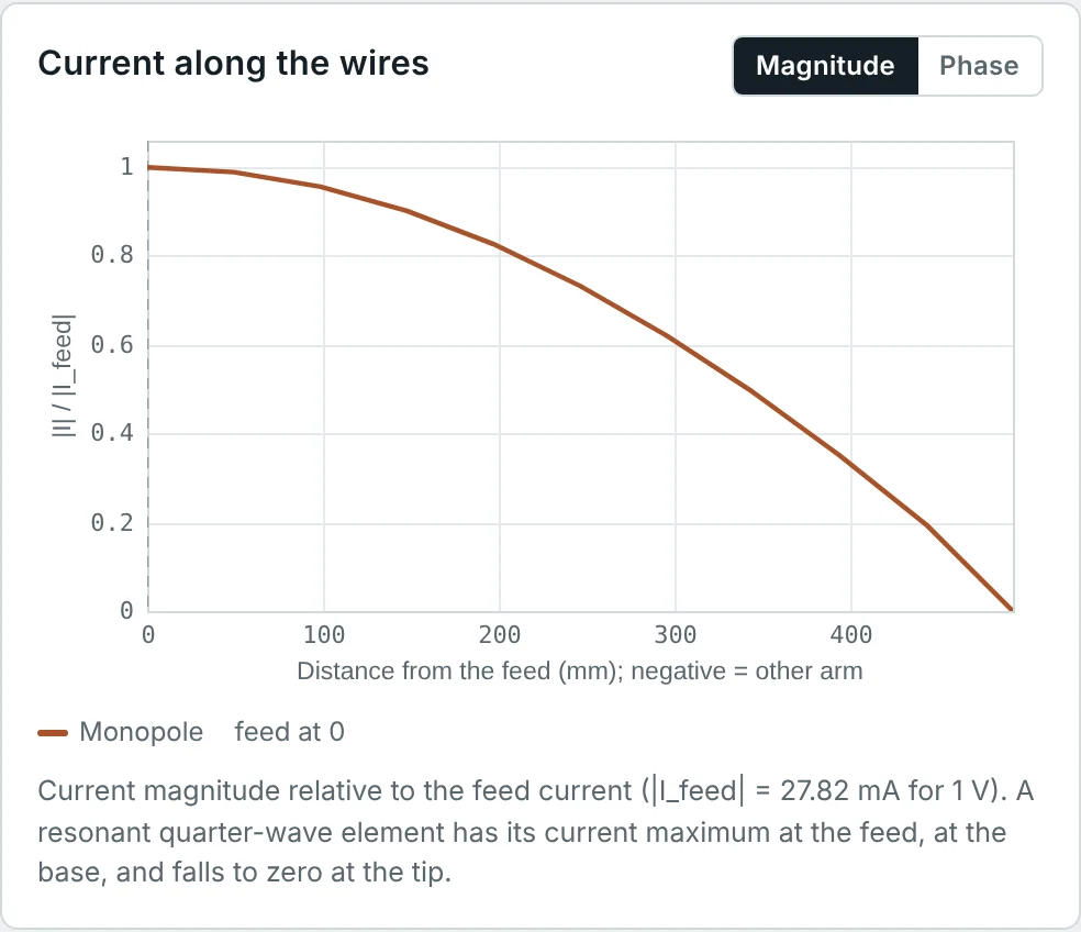
The sinusoidal approximation is excellent for thin wires (diameter below about λ/100). It slightly misrepresents the current near the feed gap and fails to predict the input reactance accurately, which is why numerical methods are used for impedance, while the simple sine gives patterns that are almost indistinguishable from exact solutions.

Radiation from a Short Dipole: The Complete Solution

The Hertzian dipole is a current element of length L ≪ λ along the z-axis carrying a uniform current I. It is the building block of all antennas: any current distribution can be treated as a sum of Hertzian dipoles. Because L is tiny, R ≈ r in the retarded-potential integral and the integral is simply I·L:

Step 1 — vector potential

A_{z} = \frac{μ I L}{4 π r} e^{- j k r} A_{r} = A_{z} \cos θ, A_{θ} = - A_{z} \sin θ

Converting the z-directed vector to spherical components prepares it for the curl in spherical coordinates.

Taking the curl, H = (1/μ)∇ × A, only the φ component survives:

Step 2 — magnetic field

H_{φ} = \frac{1}{μ r} [\frac{\partial}{\partial r} (r A_{θ}) - \frac{\partial A_{r}}{\partial θ}] = j \frac{k I L \sin θ}{4 π r} [1 + \frac{1}{j k r}] e^{- j k r} H_{r} = H_{θ} = 0

The magnetic field circles the wire, as Ampère's law requires. The 1/(jkr) term is the familiar Biot–Savart field of a short current element; the 1 term is new — it exists only because of retardation.

Outside the source J = 0, so the Ampère–Maxwell law gives E = (1/jωε)∇ × H:

Step 3 — electric field

E_{r} = η \frac{I L \cos θ}{2 π r^{2}} [1 + \frac{1}{j k r}] e^{- j k r}

E_{θ} = j η \frac{k I L \sin θ}{4 π r} [1 + \frac{1}{j k r} - \frac{1}{{(k r)}^{2}}] e^{- j k r} E_{φ} = 0

These are exact for a Hertzian dipole at every distance. The term 1/(kr)² in E_θ, together with E_r, is the quasi-static field of an electric dipole (charges ±q = ±I/jω at the ends), falling as 1/r³.

Three kinds of field

Each field contains terms that fall as 1/r, 1/r² and 1/r³. Factoring out the common 1/r, their relative sizes inside the brackets are 1, 1/(kr) and 1/(kr)²:

Term	Varies as	Name	Physical meaning
1	1/r	Radiation field	E_θ and H_φ in phase, \|E_θ/H_φ\| = η: carries real power to infinity
1/(jkr)	1/r²	Induction field	Biot–Savart magnetic field of the current; 90° out of phase with the radiation term
1/(kr)²	1/r³	Electrostatic (quasi-static) field	The field of the oscillating dipole charges; stores electric energy

All three are equal in magnitude at kr = 1, that is at r = λ/2π ≈ 0.16 λ. Well inside this radius the stored (reactive) terms dominate; well outside it, only the radiation term remains. Part 3 builds the formal near-field and far-field boundaries on this result.

The far-field limit

For kr ≫ 1, drop every term except the 1/r terms:

Far field of a Hertzian dipole

E_{θ} \approx j η \frac{k I L}{4 π r} \sin θ e^{- j k r} H_{φ} \approx \frac{E_{θ}}{η} E_{r} \approx 0

The far field is transverse (no radial component), E and H are in phase and in the ratio η, and the angular dependence sin θ is separate from the distance dependence e^(−jkr)/r. These are the properties of a spherical wave that looks locally like a plane wave.

Radiated power from the far field

The time-average Poynting vector of the far field is radial, S_r = |E_θ|²/(2η). Integrating over a sphere reproduces the Larmor-based result of Part 1, now obtained purely from the fields:

Radiated power of a Hertzian dipole

P_{rad} = \int_{0}^{2 π} \int_{0}^{π} \frac{{| E_{θ} |}^{2}}{2 η} r^{2} \sin θ d θ d φ = \frac{η k^{2} {| I |}^{2} L^{2}}{32 π^{2}} \cdot 2 π \cdot \frac{4}{3} = \frac{η π}{3} {(\frac{L}{λ})}^{2} {| I |}^{2}

If the full fields (including the 1/r² and 1/r³ terms) are used, the complex Poynting vector also has an imaginary part that grows without limit as r → 0. That imaginary part is the reactive power stored near the antenna; it appears in the input impedance as the reactance X_A (Part 7).

Near Field and Far Field of an Antenna

A compact way to see the transition is the wave impedance Z_w = E_θ/H_φ. Dividing the exact expressions above:

Wave impedance of an electric dipole and of a small loop

Z_{w}^{dipole} = η \frac{1 + \frac{1}{j k r} - \frac{1}{{(k r)}^{2}}}{1 + \frac{1}{j k r}} Z_{w}^{loop} = \frac{η^{2}}{Z_{w}^{dipole}}

The small loop is the electromagnetic dual of the short dipole (E and H swap roles), so its wave impedance is the "inverse". For kr ≪ 1, |Z_w| ≈ η/(kr) for the dipole (high impedance, mostly E) and η·kr for the loop (low impedance, mostly H).

Fig 2 — Magnitude of the wave impedance relative to η = 377 Ω against kr = 2πr/λ: electric dipole (high-impedance near field) and small loop (low-impedance near field) both approach 377 Ω in the far field

Short electric dipole |Zw|/ηSmall loop |Zw|/η

Fig 2 explains why shielding, RF-exposure assessment and near-field communication all depend on distance. A high-impedance near field (dipole) is mostly electric and is stopped well by a thin conductor; a low-impedance near field (loop) is mostly magnetic and passes through thin non-magnetic metal. Beyond a few λ/2π, both fields settle to 377 Ω and become ordinary radiation.

Electromagnetic Wave Propagation from an Antenna

In the far field, every antenna produces a spherical wave of the same general form:

General far field of any antenna

E (r, θ, φ) \approx \frac{e^{- j k r}}{r} F (θ, φ) H = \frac{1}{η} \hat{r} \times E S_{av} = \frac{{| E |}^{2}}{2 η}

The vector F(θ, φ) contains everything specific to the antenna: its pattern (Part 4) and its polarization (Part 11). The factor e^(−jkr)/r is universal: a phase that advances by 2π every wavelength and an amplitude that falls as 1/r.

Because the power density falls as 1/r² while the area of a sphere grows as r², the total power crossing any sphere in the far field is constant — this is the conservation statement behind the inverse-square law and behind the free-space path loss of Part 13. At large distances, a small patch of the spherical wavefront is very nearly flat, which is why a distant receiving antenna can treat the incoming wave as a plane wave.

Radiation from Different Antenna Geometries

Dipole of any length

A finite dipole is a chain of Hertzian dipoles, each of strength I(z′)dz′, located at z′. In the far field the distance from each element is R ≈ r − z′cos θ in the phase, and R ≈ r in the amplitude. Adding them up with the sinusoidal current gives a closed form:

Far field of a centre-fed dipole of length L — derivation

E_{θ} = j η \frac{k \sin θ}{4 π r} e^{- j k r} \int_{- L / 2}^{L / 2} I (z^{'}) e^{j k z^{'} \cos θ} d z^{'} = j η \frac{I_{m} e^{- j k r}}{2 π r} [\frac{\cos (\frac{k L}{2} \cos θ) - \cos (\frac{k L}{2})}{\sin θ}]

The integral of a sine times a complex exponential is elementary; the sin θ in front cancels against sin²θ produced by the integration, leaving one sin θ in the denominator. For L = λ/2 the bracket becomes cos(π/2·cos θ)/sin θ, the half-wave pattern of Part 4.

Fig 3 — Normalized far-field patterns of centre-fed dipoles (wire vertical, 0°–180°), linear field scale. Longer dipoles have narrower beams until, beyond 1.25 λ, the main lobe splits

L = λ/2L = λ

L = 1.25 λL = 1.5 λ

Length L	Main beam	HPBW	Directivity	Comment
≪ λ (Hertzian)	Broadside	90°	1.50 (1.76 dBi)	sin θ pattern
λ/2	Broadside	78.1°	1.64 (2.15 dBi)	Reference antenna; R ≈ 73 Ω
λ	Broadside	47.8°	2.41 (3.82 dBi)	Current minimum at the feed: very high input impedance
1.25 λ	Broadside	32.6°	3.28 (5.16 dBi)	Maximum broadside directivity of a single wire ("extended double Zepp")
1.5 λ	42.6° and 137.4° from the wire	32.8°	2.23 (3.48 dBi)	Broadside lobe now smaller than the oblique lobes

Loops, slots and patches

Other geometries follow the same rule — the current (or the aperture field) determines the radiation:

Small loop: a loop of area A carrying a uniform current is a magnetic dipole. Its fields are the dual of the short dipole: E_φ ∝ sin θ, with radiation resistance R_r = 31 200 (A/λ²)² Ω — even smaller than a short dipole of similar size.
Slot in a metal sheet: by Babinet's principle, a slot is the dual of a strip dipole of the same shape. Its electric field is across the slot, and Z_slot·Z_dipole = η²/4.
Microstrip patch: the patch is a resonant cavity. Its fringing fields at the two radiating edges act as two slots half a wavelength apart, whose fields add broadside to the board (Part 14).
Horns and reflectors: the fields across the aperture radiate like a sum of Huygens sources; the larger the aperture in wavelengths, the narrower the beam (Part 12).

Factors Affecting Antenna Radiation

Factor	Effect on radiation	Where it is treated
Electrical size (L/λ)	R_r ∝ (L/λ)² for small antennas; pattern shape and directivity change with length (Fig 3)	Parts 1, 7, 10
Current distribution	Sets the pattern through the radiation integral; tapering reduces side lobes	Part 4
Frequency	Changes the electrical size of a fixed structure; impedance and pattern vary across the band	Part 10
Conductor and dielectric losses	Turn some input power into heat instead of radiation	Part 9
Ground and nearby objects	Reflections add to the direct radiation and reshape the pattern (image theory)	Below, and Part 14
Feed and balun	Unbalanced feeding causes current on the cable shield, which radiates and distorts the pattern	Part 8
Polarization of the currents	Sets the orientation of E in the far field	Part 11

The effect of ground: image theory

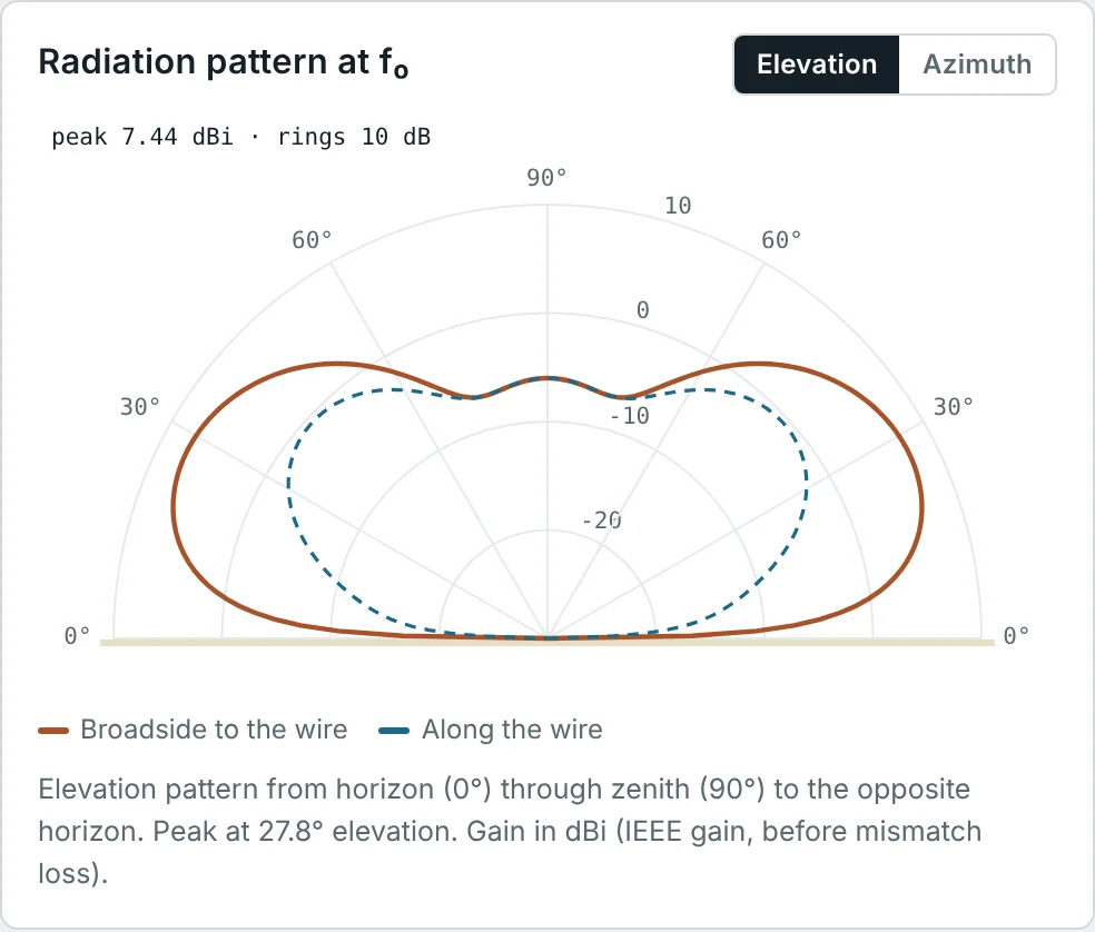
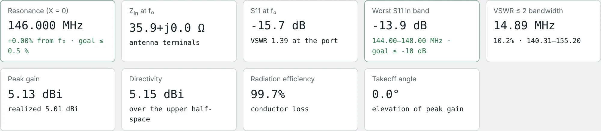
A perfectly conducting plane forces the tangential electric field to zero at its surface. The fields above the plane are then exactly those of the real antenna plus a mirror-image antenna below the plane. A vertical monopole of height h over ground is therefore equivalent, above the ground, to a dipole of length 2h; it radiates the same fields into half the space, so it has half the radiation resistance and twice the directivity of the dipole. The calculator confirms this: a 146 MHz quarter-wave monopole has Z_in = 35.9 Ω (half of the dipole's 71.9 Ω) and 5.13 dBi peak gain (≈ 2.15 + 3 dB).

For a horizontal dipole at height h above ground, the image current is reversed, and the two form a two-element array. The elevation pattern is multiplied by the array factor |2 sin(kh sin Δ)|, where Δ is the elevation angle above the horizon. The first maximum is where kh sin Δ = π/2:

Take-off angle of a horizontal dipole over a perfect ground

AF (Δ) = 2 | \sin (k h \sin Δ) | \sin Δ_{max} = \frac{λ}{4 h}

At h = λ/2, Δ_max = 30°. A higher antenna gives a lower take-off angle, which is what long-distance HF communication needs. A perfect ground also doubles the field in the peak direction: the directivity rises from 2.15 dBi to 8.4 dBi at h = λ/2.

Elevation pattern of a horizontal half-wave dipole half a wavelength above average ground: a main lobe peaking near 28 degrees elevation and a small lobe overhead — A 7.15 MHz copper dipole λ/2 above average earth: the ground reflection creates a lobe at 27.8° elevation and 7.44 dBi peak gain. Real ground is not a perfect conductor, so the angle is a little lower than the 30° of the ideal formula, and the ground absorbs about 22% of the power (Part 9). Try it in the Dipole & Monopole Antenna Calculator →

Worked Examples

Radiation Field of an Accelerating Electron

Problem: An electron accelerates at a = 10¹⁸ m/s² (typical in an X-ray tube target). Find the radiation field 1 m away, perpendicular to the acceleration, and the total power it radiates.

E_{rad} = \frac{1.602 \times 10^{- 19} \times 10^{18}}{4 π (8.854 \times 10^{- 12}) {(3 \times 10^{8})}^{2} (1)} = 1.60 \times 10^{- 8} V/m

P = \frac{q^{2} a^{2}}{6 π ε_{0} c^{3}} = 5.7 \times 10^{- 18} W

Answer: 16 nV/m and 5.7 × 10⁻¹⁸ W per electron

One electron radiates almost nothing. An antenna works because ~10²³ electrons per cm³ accelerate together, so their fields add coherently and the power scales as the square of the total current.

Relative Size of the Three Field Terms

Problem: For a Hertzian dipole, compare the magnitudes of the 1/r, 1/r² and 1/r³ terms of E_θ at kr = 0.1, 1 and 10.

kr	r	Radiation (1)	Induction (1/kr)	Static (1/(kr)²)	Dominant
0.1	0.016 λ	1	10	100	Static, 99% of \|E_θ\|
1	0.16 λ	1	1	1	All equal
10	1.6 λ	1	0.1	0.01	Radiation

Answer: 1 : 10 : 100 at kr = 0.1, equal at kr = 1, 1 : 0.1 : 0.01 at kr = 10

At kr = 10 the reactive terms still alter the field by about 1% in magnitude and a few degrees in phase — the reason the precise far-field boundary of Part 3 depends on how much error is acceptable.

Where the Radiation Term Takes Over

Problem: Find the distance r = λ/2π at 146 MHz (a VHF handheld) and at 13.56 MHz (NFC, RFID). Which region does each system operate in?

r_{146} = \frac{2.053}{2 π} = 0.327 m r_{13.56} = \frac{22.11}{2 π} = 3.52 m

Answer: 33 cm at 146 MHz; 3.5 m at 13.56 MHz

A handheld radio is in the radiation zone a metre away, while an NFC reader 4 cm from a card is 90 times closer than λ/2π — deep in the magnetic near field of a loop. NFC couples like a loosely coupled transformer, not like a radio link.

Wave Impedance in the Near Field

Problem: Evaluate the wave impedance of a short electric dipole at kr = 0.5. Is it inductive or capacitive?

Z_{w} = 377 \frac{1 - j 2 - 4}{1 - j 2} = 377 \frac{- 3 - j 2}{1 - j 2} = 377 (0.2 - j 1.6) = 75 - j 603 Ω

Answer: Z_w = 75 − j603 Ω, |Z_w| = 607 Ω at −82.9° (capacitive)

The large negative reactance shows that the space around a short dipole stores mostly electric energy, as a capacitor does. Correspondingly, a short dipole's input impedance is strongly capacitive (Part 7). The dual small loop has Z_w = η²/Z_w ≈ 29 + j232 Ω: inductive.

Radiated Power by Field Integration

Problem: A λ/20 current element carries 2 A peak. Compute the radiated power by integrating the far-field Poynting vector, and find R_r.

P_{rad} = \frac{120 π \cdot π}{3} {(\frac{1}{20})}^{2} 2^{2} = 40 π^{2} \times 0.0025 \times 4 = 3.95 W R_{r} = \frac{2 \times 3.95}{4} = 1.97 Ω

Answer: 3.95 W radiated, R_r = 1.97 Ω

The ∫sin³θ = 4/3 factor shows that a sin²θ power pattern puts 2/3 of the power that an isotropic source of the same peak would radiate — which is why its directivity is 1.5 (Part 6).

Field Strength of a Half-Wave Dipole

Problem: A half-wave dipole carries I_m = 1 A peak at its feed. Using the dipole far-field formula, find |E| broadside at 1 km and the total radiated power (Part 6 gives P_rad = 36.57 I_m² W).

| E_{θ} | = \frac{η I_{m}}{2 π r} \cdot \frac{\cos (\frac{π}{2} \cos 90 °)}{\sin 90 °} = \frac{60 I_{m}}{r} = 60 mV/m P_{rad} = 36.6 W

Answer: 60 mV/m at 1 km; 36.6 W radiated

The rule "E = 60 I/r broadside" for a half-wave dipole is worth remembering: 60 = η/2π. Equivalently, the radiation resistance referred to the current maximum is 2 × 36.57 = 73.1 Ω.

Pattern of a Full-Wave Dipole

Problem: For L = λ, simplify the dipole pattern and find its half-power beamwidth.

\frac{k L}{2} = π F (θ) = \frac{\cos (π \cos θ) + 1}{2 \sin θ} = \frac{\cos^{2} (\frac{π}{2} \cos θ)}{\sin θ}

Solving F(θ_h) = 0.707 numerically gives θ_h = 66.1°, so HPBW = 2(90° − 66.1°) = 47.8°. Integrating F² gives D = 2.41 (3.82 dBi).

Answer: F = cos²(π/2·cos θ)/sin θ; HPBW = 47.8°, D = 3.82 dBi

The full-wave pattern is the half-wave pattern multiplied by cos(π/2·cos θ): two half-wave dipoles end to end, in phase — a two-element collinear array (Part 4).

Monopole Impedance by Image Theory

Problem: The 146 MHz dipole in the calculator has Z_in = 71.9 Ω and D = 2.14 dBi. Predict the input impedance and directivity of a quarter-wave monopole on an ideal ground plane, and compare with the calculator.

Z_{mono} = \frac{Z_{dipole}}{2} = 36.0 Ω D_{mono} = 2 D_{dipole} \Rightarrow 2.14 + 3.01 = 5.15 dBi

Answer: 36 Ω and 5.15 dBi; the calculator gives 35.9 Ω and 5.15 dBi

The same voltage drives half the structure, and the same current produces the same fields in half the space with half the radiated power. A real vehicle roof or radial set is finite, so real monopoles have a slightly tilted beam and lower gain.

Monopole calculator readouts: resonance at 146 MHz, Zin 35.9 ohms, S11 minus 15.7 dB, peak gain 5.13 dBi, directivity 5.15 dBi, radiation efficiency 99.7 percent — Calculator readouts for the 146 MHz quarter-wave monopole: Z_in = 35.9 Ω and 5.15 dBi directivity, exactly half the dipole impedance and twice its directivity. Try it in the Dipole & Monopole Antenna Calculator →

Take-Off Angle of an HF Dipole

Problem: A 7.15 MHz dipole is mounted horizontally at h = 21 m. Find the elevation angle of maximum radiation over a perfect ground. What height gives a 15° take-off angle?

λ = 41.9 m \sin Δ_{max} = \frac{41.9}{4 \times 21} = 0.499 \Rightarrow Δ_{max} = 29.9 ° h = \frac{λ}{4 \sin 15 °} = 40.5 m

Answer: 29.9° (the calculator, over average earth, gives 27.8°); about 40 m for 15°

Real earth reflects less than a perfect conductor and with a different phase, which lowers the angle slightly, fills in the overhead null and costs about 2 dB of gain.

Radiation Resistance of a Small Loop

Problem: A single-turn loop of 10 cm diameter operates at 30 MHz. Find R_r = 31 200 (A/λ²)² and compare with a 10 cm short dipole at the same frequency (R_r = 20π²(L/λ)²).

A = π {(0.05)}^{2} = 7.85 \times 10^{- 3} m² R_{loop} = 31 200 {(\frac{7.85 \times 10^{- 3}}{100})}^{2} = 1.9 \times 10^{- 4} Ω R_{dipole} = 20 π^{2} {(0.01)}^{2} = 0.020 Ω

Answer: 0.19 mΩ for the loop, 20 mΩ for the dipole — about 100 times less

Loop radiation resistance falls as the fourth power of size (A²), dipole resistance as the square. Small transmitting loops therefore need very low-loss construction (wide copper tube, vacuum capacitor) and multiple turns (R_r ∝ N²) — while for receiving, the loop's low-impedance magnetic near field makes it less sensitive to nearby electric noise.

Summary

Radiation comes from accelerating charge; an accelerating charge has a transverse field q a sin θ/(4πε₀c²r) that falls as 1/r and carries away the Larmor power.
Antenna fields follow from the retarded vector potential A = (μ/4π)∫J e^(−jkR)/R dV, the basis of every pattern and every numerical solver.
A Hertzian dipole has exact fields with 1/r (radiation), 1/r² (induction) and 1/r³ (quasi-static) terms; they are equal at kr = 1, r = λ/2π.
In the far field, E_θ = jηkIL sin θ e^(−jkr)/(4πr), H_φ = E_θ/η, and P_rad = (ηπ/3)(L/λ)²|I|².
The wave impedance is high (capacitive) near a dipole and low (inductive) near a loop; both tend to 377 Ω beyond a few λ/2π.
A centre-fed dipole of length L has the pattern [cos(kL/2·cos θ) − cos(kL/2)]/sin θ; the beam narrows up to L = 1.25 λ and then splits.
Current distribution, electrical size, losses, feed and especially ground shape the radiation; image theory explains monopoles (half the impedance, twice the directivity) and the take-off angle of horizontal antennas.

The fields around an antenna change character with distance. Part 3: Antenna Near Field and Far Field divides that space into the reactive near field, the radiating near field and the far field, and derives the boundaries used in measurement and RF-exposure work.

Put It Into Practice

Use the NEXT ANTENNAS calculators to apply the ideas from this article to real antennas.

Wire Antennas Dipole & Monopole Antenna Calculator Method of Moments design of dipoles, inverted-Vs and monopoles: length, impedance, S11, current, gain and 3D patterns. Open calculator → Wire Antennas Monopole & Ground Plane Calculator Quarter-wave monopoles and ground-plane antennas with radials: length, impedance and radial angle. Open calculator → Antenna & Signal Wavelength / Frequency Calculator Convert between frequency and wavelength in free space and in dielectrics. Open calculator → All Tools All RF Calculators Browse every NEXT ANTENNAS calculator for RF, microwave and antenna design. Open calculator →