What Is an Antenna?
The IEEE Standard Definitions of Terms for Antennas (IEEE 145) defines an antenna as "that part of a transmitting or receiving system that is designed to radiate or to receive electromagnetic waves." In plainer words: an antenna is a conductor (or a dielectric, or a slot in a conductor) shaped so that the currents flowing on it launch a wave into space, or so that an arriving wave drives currents on it.
Inside a cable the signal is a guided wave: its fields are confined between two conductors and it can only travel along the cable. In free space the signal is a radiated wave: its fields spread outward in all directions at the speed of light. The antenna is the structure that converts one into the other, so it is often described as a transition region between a transmission line and free space.
If you have read our introductory article Antenna Basics, this series now builds the full theory: how radiation happens (Part 2), where the far field begins (Part 3), how energy is distributed in direction (Parts 4–6), how the antenna looks to the circuit that feeds it (Parts 7–10), polarization and aperture (Parts 11–12), and finally the complete radio link (Part 13).
Why Are Antennas Needed in Wireless Communication?
A transmitter produces an oscillating voltage at a radio frequency. Connected to an ordinary closed circuit — a resistor, a coaxial cable — almost none of that power leaves as radiation: the fields stay tightly bound to the conductors and the power is either dissipated or returned to the source. Three facts explain why a special structure is needed.
1. Free space has its own impedance
A plane wave in free space carries electric and magnetic fields in a fixed ratio, the intrinsic impedance of free space, derived in our wave-equation article:
2. Radiation needs a size comparable with the wavelength
A structure radiates efficiently only when its currents are spread over a distance comparable with the wavelength. A circuit board trace 1 cm long at 50 Hz is 6 × 10⁻⁹ wavelengths long; its fields simply collapse back into the circuit each cycle. The same trace at 7.5 GHz is a quarter-wavelength long and radiates strongly — which is why high-speed digital boards cause interference. Example 4 puts numbers on this.
| Service | Frequency | Wavelength λ | Half-wave dipole λ/2 |
|---|---|---|---|
| AM broadcast | 1 MHz | 300 m | 150 m (a quarter-wave mast, 75 m, is used instead) |
| HF amateur 40 m band | 7.15 MHz | 41.9 m | ≈ 20.6 m |
| FM broadcast | 100 MHz | 3.00 m | 1.50 m |
| VHF two-way radio | 146 MHz | 2.05 m | ≈ 0.98 m |
| Cellular / LTE | 1.8 GHz | 16.7 cm | 8.3 cm |
| Wi-Fi, Bluetooth | 2.45 GHz | 12.2 cm | 6.1 cm |
| 5G NR (FR2) | 28 GHz | 10.7 mm | 5.4 mm |
| Automotive radar | 77 GHz | 3.9 mm | 1.9 mm |
3. Waves reach places cables cannot
Radio waves cross oceans, reach moving vehicles and satellites, penetrate walls, and serve millions of users from one transmitter. Above about 100 kHz, a radiated wave loses power only as 1/r² with distance (the free-space spreading of Part 5), while a cable loses a fixed number of decibels per metre. For long distances and for mobility, an antenna is not just convenient — it is the only option.
Basic Working Principle of an Antenna
Static charges produce static electric fields; steady currents produce static magnetic fields. Neither radiates. Radiation requires accelerating charge, or equivalently a time-varying current. Part 2 explains the field picture in detail; here we derive how much power is radiated, starting from the simplest possible source.
Radiation from one accelerating charge
A charge q moving with acceleration a radiates a total power given by the Larmor formula:
From one charge to a current element
An antenna does not carry one charge but a current: an enormous number of electrons sloshing back and forth. Consider a short wire of length L (much shorter than λ) carrying a uniform current I(t). The charge in the wire moves with velocity v, and the current is the charge per unit length times v, so q·v summed over the wire equals L·I. Differentiating with respect to time:
For a sinusoidal current I(t) = I₀ cos ωt, dI/dt = −ωI₀ sin ωt, and the time average of sin² ωt is ½. Using μ₀c = η and ω/c = k = 2π/λ gives the average radiated power:
Radiation resistance
From the circuit's point of view, power that leaves as radiation is lost just as if it were burned in a resistor. Writing P_rad = ½ I₀² R_r defines the radiation resistance R_r:
R_r grows rapidly with electrical length. A half-wave dipole, whose current is a half-cycle of a sine wave, reaches about 73 Ω (derived in Part 6 and Part 7) — conveniently close to the 50 Ω and 75 Ω of standard cables, which is one reason the half-wave dipole is the reference antenna of radio engineering.
How Electrical Signals Are Converted into Electromagnetic Waves
A classic way to see how a transmission line becomes an antenna is to open it up. In a two-wire line the two conductors carry equal and opposite currents a small fraction of a wavelength apart. Their fields cancel at any distance much greater than the spacing, so the line guides energy but does not radiate. Bend the last quarter-wavelength of each wire outward by 90°, and the currents on the two arms now flow in the same direction in space. Their fields add instead of cancelling: the line has become a half-wave dipole.
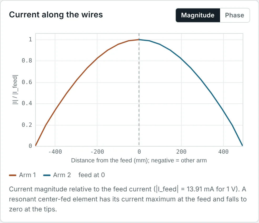
The current on the finished dipole is a standing wave: zero at the open ends, where charge can go no further, and maximum at the feed a quarter-wavelength away. The calculator screenshot below is a Method of Moments solution for a 146 MHz dipole and shows exactly this half-cycle shape. The charges oscillate along each arm, constantly accelerating and decelerating, and the fields they generate detach from the wire and travel outward — the subject of Part 2.
How Electromagnetic Waves Are Received by an Antenna
Receiving is the same process in reverse. A wave arriving at a wire exerts a force qE on the free electrons. The tangential component of the incident electric field along the wire drives a current, and a voltage appears across the antenna terminals. With nothing connected (open circuit), that voltage is proportional to the incident field:
Connected to a receiver, the antenna behaves as a voltage source V_oc with an internal impedance equal to its own input impedance Z_A (this is a consequence of reciprocity). Maximum power reaches the receiver when the receiver impedance is the complex conjugate of Z_A. With a lossless antenna, Z_A = R_r + jX_A, the received power under conjugate match is
How much power does a small dipole capture?
Combine the two results for a short dipole. With ℓ_e = L/2 and R_r = 20π²(L/λ)²:
Part 12 generalizes this to every antenna: A_e = Dλ²/4π, with D = 1.5 for a short dipole, which gives exactly 3λ²/8π. The effective aperture is the bridge between the incoming power density and the received power, and it is the receiving half of the Friis equation in Part 13.
Transmitting Antennas vs. Receiving Antennas
The reciprocity theorem, which follows from Maxwell's equations for linear, passive, isotropic media, states that if a current source at the terminals of antenna A produces a voltage at the terminals of antenna B, the same source at B produces the same voltage at A. Its consequences for a single antenna are that the radiation pattern, directivity, gain, input impedance and polarization are identical in transmit and receive.
| Aspect | Transmitting antenna | Receiving antenna |
|---|---|---|
| Energy flow | Terminals → space | Space → terminals |
| Pattern, gain, polarization | Identical (reciprocity) | |
| Input impedance | Identical — the same Z_A appears in both equivalent circuits | |
| Power level | Watts to megawatts: voltage breakdown, heating and passive intermodulation matter | Picowatts to microwatts: noise and sensitivity matter |
| Efficiency priority | Every lost dB is lost transmitter power | Losses add thermal noise; matters most when external noise is low (satellite, GNSS) |
| Exceptions | Active antennas (with amplifiers), antennas containing ferrites or plasmas, and some reconfigurable antennas are not reciprocal | |
Reciprocity is extremely useful in practice: an antenna is usually measured in whichever mode is easier, and the result holds for the other. The pattern measurements in Part 4 and the gain measurements in Part 6 rely on it.
The Antenna as a Transducer: Equivalent Circuit
To the circuit connected to it, an antenna is a two-terminal load (when transmitting) or a source (when receiving). Its input impedance is
In the transmitting circuit, the current I_A through the antenna splits the accepted power into a radiated part, ½|I_A|²R_r, and a loss, ½|I_A|²R_L. When Z_g ≠ Z_A*, part of the available power never enters the antenna; this mismatch is described by the reflection coefficient of Part 8. The full chain from transmitter to radiated power is therefore
Basic Components of an Antenna System
The radiating element is only one part of what engineers call "the antenna". A complete antenna system includes everything between the radio's connector and free space:
| Component | Function | Typical examples |
|---|---|---|
| Transmission line (feeder) | Carries the guided wave between radio and antenna with minimum loss | Coaxial cable, microstrip, waveguide, twin-lead |
| Matching network | Transforms Z_A to the line impedance (Part 8) | L-networks, quarter-wave transformers, stubs, gamma match |
| Balun | Connects a balanced antenna (dipole) to an unbalanced line (coax), stopping current on the outside of the shield | Current (choke) balun, sleeve balun, ferrite beads |
| Radiating element | Carries the radiating currents | Dipole, monopole, patch, slot, horn aperture |
| Ground plane or reflector | Provides an image (monopole), a reflector for directivity (patch, Yagi), or focuses the beam (dish) | Vehicle roof, PCB ground, reflector screen, parabolic dish |
| Feed network (arrays) | Splits power to many elements with set amplitudes and phases (Part 4) | Corporate feeds, phase shifters, beamforming ICs |
| Radome and mounting | Protects from weather; positions and orients the antenna | Fibreglass radomes, masts, brackets |
Each component can cost decibels. A typical base-station installation loses 2–3 dB in its feeder alone, which is why modern systems place the radio electronics at the top of the mast, directly behind the antenna.
Applications of Antennas in Everyday Life
| Application | Frequency | Typical antenna | Main requirement |
|---|---|---|---|
| AM / FM broadcast | 0.5–1.7 MHz / 88–108 MHz | Tower monopole / dipole arrays | High power, omnidirectional coverage |
| Smartphones | 0.6–6 GHz, 24–40 GHz | PIFAs, monopoles in the frame, mm-wave patch arrays | Small size, many bands, close to the body |
| Cellular base stations | 0.7–3.8 GHz | Dual-polarized panel arrays, massive MIMO | Sector coverage, beam steering, tilt |
| Wi-Fi and Bluetooth | 2.4, 5, 6 GHz | Dipoles, printed monopoles, chip antennas | Low cost, omnidirectional |
| GNSS (GPS, Galileo) | 1.2–1.6 GHz | Ceramic patch, quadrifilar helix | Right-hand circular polarization (Part 11) |
| Satellite TV and broadband | 10.7–30 GHz | Parabolic dish, flat phased arrays | Very high gain, narrow beam |
| Radar | 1–100 GHz | Reflectors, slotted waveguides, phased arrays | High gain, low side lobes, steering |
| RFID and NFC | 13.56 MHz, 860–960 MHz | Loops (near-field coupling), meandered dipoles | Tiny, cheap, tolerant of nearby objects |
| Medical and IoT | 0.4–2.5 GHz | Implantable and wearable antennas | Operation in or on lossy tissue |
Classification of Antennas Based on Their Structure
Antennas are most often grouped by how their radiating currents or fields are formed. Part 14 describes each family in detail; this overview introduces the vocabulary used throughout the series.
| Family | How it radiates | Examples | Typical gain |
|---|---|---|---|
| Wire antennas | Currents on thin conductors | Dipole, monopole, loop, helix, Yagi-Uda | −5 to 15 dBi |
| Aperture antennas | Fields across an opening | Horn, open waveguide, slot | 5 to 25 dBi |
| Microstrip (printed) antennas | Fringing fields at the edges of a resonant patch | Rectangular and circular patches, printed dipoles | 3 to 8 dBi per element |
| Reflector antennas | A feed illuminates a large shaped reflector | Parabolic dish, corner reflector, Cassegrain | 20 to 70 dBi |
| Lens and dielectric antennas | A dielectric shapes the phase front, or resonates | Lens horns, dielectric resonator antennas | 5 to 40 dBi |
| Arrays | Many elements combined with controlled amplitude and phase | Phased arrays, massive MIMO panels | 10 to 40 dBi |
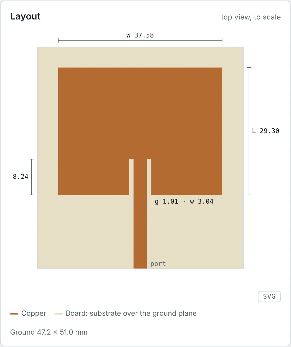
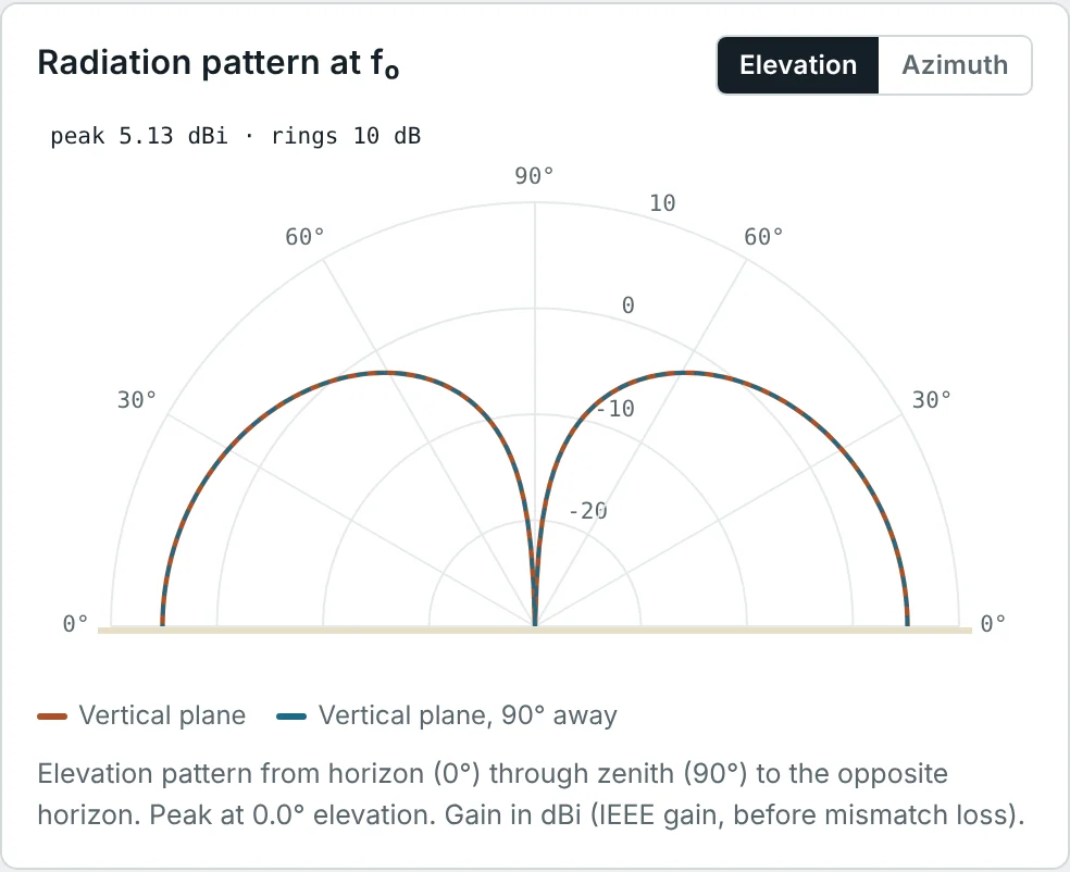
Antennas are also classified by bandwidth (narrowband, broadband, ultra-wideband — Part 10), by pattern (isotropic, omnidirectional, directional — Part 4), by polarization (linear or circular — Part 11), and by whether they are passive, active or reconfigurable. Our Antenna Types learning path covers practical designs of each type.
Worked Examples
Wavelength and Half-Wave Dipole Length
Problem: Find the wavelength and the ideal half-wave dipole length at 100 MHz (FM broadcast) and at 2.45 GHz (Wi-Fi). Why is a practical dipole cut slightly shorter?
A real wire has a finite diameter, and the fringing fields at its ends make it look electrically longer. A wire cut exactly to λ/2 is slightly inductive (Z ≈ 73 + j42.5 Ω); shortening it to about 0.47–0.49 λ removes the reactance. The calculator's 146 MHz design is 0.479 λ long for a 2 mm wire (Part 7).
Radiation Resistance of a Very Short Antenna
Problem: A 10 cm wire with a uniform current is used at 30 MHz. Find its radiation resistance. If the wire and its matching coil have 1 Ω of loss resistance, what fraction of the input power is radiated?
When R_r is far below the loss resistance, most power heats the antenna. This is the fundamental difficulty of electrically small antennas, and the reason AM receivers use ferrite rods and why the efficiency of tiny IoT antennas is often 10–30% (Part 9).
Power Radiated by a Current Element
Problem: A 1 m current element carries a 1 A peak current at 10 MHz. Using the Larmor-based derivation, find the radiated power and the radiation resistance.
Doubling the frequency to 20 MHz halves λ, doubles L/λ and quadruples both numbers: radiated power rises as f² for a fixed current element, the ω² of the Larmor formula in disguise.
Why a Power Line Is a Poor Antenna
Problem: A 100 m straight section of a 50 Hz line carries 1000 A peak. Treating it as a current element, estimate the radiation resistance and radiated power.
Power lines are 10⁻⁵ wavelengths long, so their energy stays in the reactive near field (Part 3). The same physics says a 7.5 GHz clock harmonic on a 1 cm board trace (λ/4) radiates very efficiently.
Voltage and Power Received by a Short Dipole
Problem: A 1 m centre-fed dipole receives a 10 MHz wave with a peak field of 1 mV/m aligned with the wire. Find the open-circuit voltage and the maximum (conjugate-matched) received power. Check the result with A_e = 3λ²/8π.
A 1 m wire "captures" the power flowing through 107 m² — but only if it is conjugate-matched to 0.219 − jX_A Ω with no loss, which is practically impossible at 10 MHz. Real short receiving antennas deliver far less power; at HF that is acceptable because atmospheric noise is also picked up and still dominates (Part 9).
Using the Equivalent Circuit
Problem: A half-wave dipole cut exactly to λ/2 has R_r = 73.1 Ω and X_A = 42.5 Ω, plus R_L = 2 Ω of conductor loss. It is fed directly by a 50 Ω line. Find the radiation efficiency, the reflection coefficient and the fraction of available power that is radiated.
The mismatch costs far more (14%) than the conductor loss (2.7%). Trimming the dipole by a few percent cancels X_A and brings |Γ| below 0.2 — the subject of Parts 7 and 8.
Power Budget of an Antenna System
Problem: A 100 W transmitter feeds an antenna through cable with 2 dB loss. At the antenna |Γ| = 0.2 and the radiation efficiency is 90%. How much power is radiated?
In decibels: −2.0 dB (cable) − 0.18 dB (mismatch) − 0.46 dB (radiation efficiency) = −2.64 dB. The cable is the largest loss. (Strictly, the reflected wave also suffers cable loss on its way back, which slightly improves the match seen at the transmitter; Part 8 discusses this.)
Electric and Magnetic Fields of a Radio Wave
Problem: Far from an antenna, the power density is 1 mW/m². Find the RMS electric and magnetic field strengths.
These relations hold only in the far field, where E and H are in phase and in the ratio η₀. Close to the antenna, in the reactive near field, they do not — which is why RF-exposure surveys near antennas measure E and H separately (Part 3).
Power Captured by an Isotropic Antenna
Problem: A lossless, matched isotropic antenna (D = 1) receives a 2.45 GHz wave with power density 1 µW/m². Using A_e = λ²/4π (Part 12), find the received power.
The effective aperture of an antenna with fixed gain shrinks as λ²: at 24.5 GHz the same isotropic antenna captures 100 times less power. That λ² is the origin of the frequency term in the free-space path loss of Part 13.
Choosing an Antenna Family
Problem: Suggest an antenna family for each case: (a) a GPS receiver in a car; (b) a 12 GHz satellite TV link; (c) an FM car radio; (d) a 3.5 GHz 5G base station that must serve users in many directions; (e) a 13.56 MHz contactless payment card.
| Case | Choice | Reason |
|---|---|---|
| (a) GPS | Ceramic patch | Small, flat, right-hand circular polarization, wide beam toward the sky |
| (b) Satellite TV | Parabolic reflector | Needs ≈ 35 dBi to receive a weak signal from 36 000 km |
| (c) FM radio | Monopole (whip or glass-printed) | Omnidirectional in azimuth, vertical polarization, simple |
| (d) 5G base station | Phased array (massive MIMO) | High gain with electronically steered beams |
| (e) Payment card | Multi-turn loop | λ = 22 m, so the card works by magnetic near-field coupling, not radiation |
The choice follows from the requirements this series quantifies: gain (Part 6), polarization (Part 11), bandwidth (Part 10), size relative to λ (Parts 7 and 9) and field region (Part 3).
Summary
- An antenna is a transducer between a guided wave on a transmission line and a free-space wave with |E|/|H| = η₀ ≈ 377 Ω.
- Radiation needs accelerating charge: the Larmor formula P = μ₀q²a²/6πc becomes P_rad = 40π²(L/λ)²I₀² for a short current element.
- Radiated power appears to the circuit as a radiation resistance, R_r = 80π²(L/λ)² for uniform current and ≈ 73 Ω for a half-wave dipole; small antennas have tiny R_r.
- A receiving antenna is a voltage source V_oc = ℓ_e E with internal impedance Z_A; conjugate matching delivers |V_oc|²/8R_r. A short dipole captures the power through A_e = 3λ²/8π regardless of its length.
- Reciprocity makes pattern, gain, impedance and polarization the same in transmit and receive.
- The equivalent circuit Z_A = R_r + R_L + jX_A, together with cable loss and mismatch, determines how much transmitter power is actually radiated.
- An antenna system also includes the feeder, matching network, balun, ground plane, radome and (for arrays) the feed network.
- Antenna families — wire, aperture, printed, reflector, lens and array — differ in how their radiating currents or fields are formed.
We have treated radiation as a fact and measured it with the Larmor formula. Part 2: How Antennas Radiate Electromagnetic Waves looks inside the process: how fields detach from a wire, why the far field falls as 1/r, and how the current distribution shapes what an antenna radiates.
Put It Into Practice
Use the NEXT ANTENNAS calculators to apply the ideas from this article to real antennas.