Antenna Polarization Explained

Fig 1 — The path traced by the tip of the electric field vector in a fixed plane, viewed from behind the source with the wave travelling into the page (+z; x to the right, y down). RHCP turns clockwise in this view

Introduction to Antenna Polarization

The far field of an antenna is a transverse wave: its electric field lies in the plane perpendicular to the direction of travel (Part 3). Within that plane, the field can point in any direction and can rotate as it oscillates. Polarization describes that behaviour. It matters because a receiving antenna responds only to the component of the incoming field that matches its own polarization: a vertical dipole cannot receive a horizontally polarized wave, and a right-hand circular antenna cannot receive a left-hand circular one.

Definition of Polarization

IEEE 145 defines the polarization of a wave as "that property describing the time-varying direction and relative magnitude of the electric-field vector; specifically, the figure traced as a function of time by the extremity of the vector at a fixed location in space, and the sense in which it is traced, as observed along the direction of propagation." The polarization of an antenna in a given direction is the polarization of the wave it radiates in that direction. It generally varies with direction — an antenna that is circularly polarized on boresight is usually elliptical off axis.

The Polarization Ellipse

Any transverse field travelling along +z can be written as two orthogonal components with their own amplitudes and a relative phase δ:

General transverse field

E_{x} (t) = E_{x 0} \cos (ω t - k z) E_{y} (t) = E_{y 0} \cos (ω t - k z + δ)

Let u = E_x/E_x0 and v = E_y/E_y0 at a fixed z, and write φ = ωt − kz. Then u = cos φ and v = cos φ cos δ − sin φ sin δ. Eliminating φ: sin φ = (u cos δ − v)/sin δ, and cos²φ + sin²φ = 1 gives

Polarization ellipse — derivation

u^{2} + \frac{{(u \cos δ - v)}^{2}}{\sin^{2} δ} = 1 \Rightarrow {(\frac{E_{x}}{E_{x 0}})}^{2} - 2 \frac{E_{x} E_{y}}{E_{x 0} E_{y 0}} \cos δ + {(\frac{E_{y}}{E_{y 0}})}^{2} = \sin^{2} δ

This quadratic form is an ellipse: the general state of polarization of any single-frequency wave is elliptical. Linear and circular polarization are special cases.

The ellipse has a major axis OA, a minor axis OB and a tilt angle τ measured from the x-axis:

Axes and tilt of the polarization ellipse

O A, O B = {[\frac{1}{2} (E_{x 0}^{2} + E_{y 0}^{2} \pm \sqrt{E_{x 0}^{4} + E_{y 0}^{4} + 2 E_{x 0}^{2} E_{y 0}^{2} \cos 2 δ})]}^{1 / 2}

\tan 2 τ = \frac{2 E_{x 0} E_{y 0} \cos δ}{E_{x 0}^{2} - E_{y 0}^{2}}

"+" gives OA, "−" gives OB. τ is measured from the x-axis to the major axis; of the two solutions of tan 2τ (90° apart), the major axis is the one along which the field is larger. The axial ratio is AR = OA/OB.

Linear Polarization

When δ = 0 or π (the two components in phase or in antiphase), the ellipse collapses to a straight line: the field oscillates back and forth along a fixed direction at angle tan⁻¹(E_y0/E_x0). A single component (E_y0 = 0) is also linear. Thin wire antennas are naturally linearly polarized along the wire: the current flows along the wire, and so does the far-field E (Part 2).

Vertical and horizontal polarization

Near the ground, linear polarization is described relative to the earth's surface:

	Vertical polarization	Horizontal polarization
Antenna	Vertical whip, monopole, vertical dipole	Horizontal dipole, Yagi with horizontal elements, loop on its side
Pattern in azimuth	Omnidirectional from a single element	Figure-eight from a single dipole (needs turnstile or loop for omni)
Ground reflection at low angles	Varies strongly near the Brewster angle	Reflection coefficient ≈ −1 for all low angles
Typical use	Mobile radio, cellular (historically), AM broadcast, vehicles	TV broadcast in many regions, HF long-haul, point-to-point links

Modern cellular base stations use slant ±45° dual polarization: two orthogonal linear polarizations in one panel provide polarization diversity and allow 2×2 MIMO from a single antenna.

Circular Polarization

When the two components have equal amplitude and are 90° out of phase (E_x0 = E_y0, δ = ±π/2), OA = OB and the field vector has constant length and rotates once per cycle. In phasor form, with e^(jωt):

Circularly polarized waves travelling in +z

E_{RHCP} = E_{0} (\hat{x} - j \hat{y}) e^{- j k z} E_{LHCP} = E_{0} (\hat{x} + j \hat{y}) e^{- j k z}

At z = 0 the RHCP field is x̂ cos ωt + ŷ sin ωt: it turns from x toward y. With the wave travelling along +z, that rotation follows the fingers of the right hand when the thumb points along the direction of propagation.

Right-hand and left-hand circular polarization

IEEE defines the sense as observed along the direction of propagation — standing behind the transmitter, looking where the wave is going:

RHCPClockwise rotation viewed along the direction of propagation; right-hand rule with the thumb along propagation. Used by GPS, Galileo, most satellite telemetry.

LHCPCounter-clockwise viewed along the direction of propagation. Used for frequency reuse alongside RHCP (satellite TV) and by some GNSS ground-station links.

Beware the optics conventionClassical optics names the sense as seen by an observer facing the oncoming wave, which reverses the labels. Always state the convention.

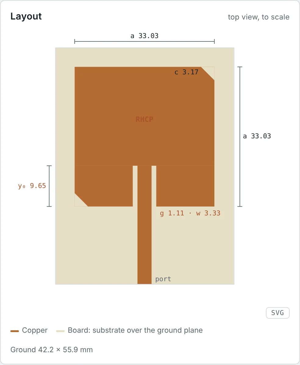
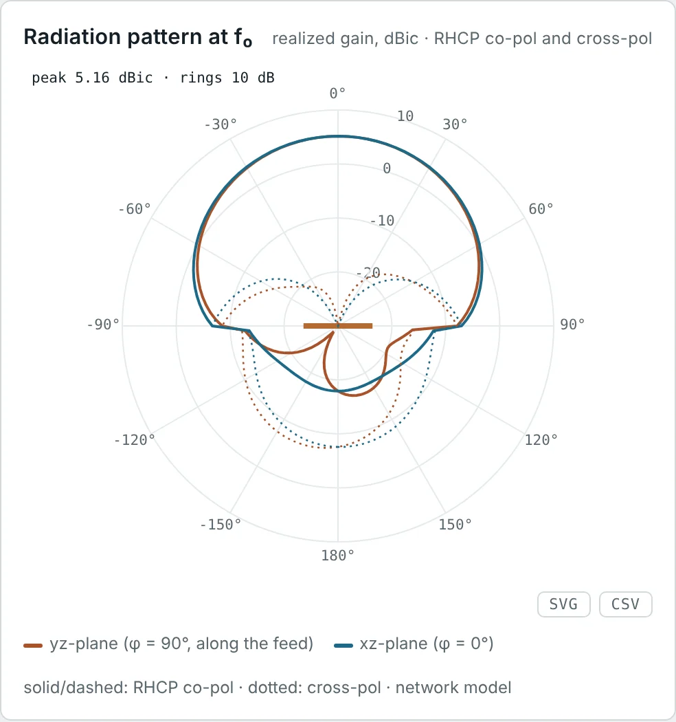
Circular polarization is produced by two orthogonal linear radiators fed with equal amplitude and 90° phase difference (crossed dipoles with a hybrid, dual-fed patches), by a single-feed patch with a perturbation that splits two modes and makes them ±45° out of phase at the centre frequency (corner truncation, as in the calculator's CP patch), by axial-mode helices and by spirals.

Layout of a square patch with two opposite corners cut off and an inset microstrip feed — A single-feed RHCP patch on RO4003C: a 33.0 mm square with two opposite corners truncated (3.2 mm legs) to split the two orthogonal modes. Try it in the Patch Antenna Calculator →

Radiation pattern cuts of the CP patch showing a broad co-polar RHCP lobe and a much weaker cross-polar LHCP pattern — Co-polar RHCP (solid) and cross-polar LHCP (dotted) patterns in two planes; on boresight the cross-polar level is 44 dB below the co-polar. Try it in the Patch Antenna Calculator →

Elliptical Polarization

Every other combination of amplitudes and phase gives an ellipse. In practice "circularly polarized" antennas are always slightly elliptical, and "linearly polarized" antennas have a small orthogonal component. Elliptical polarization is fully described by three numbers: the axial ratio, the tilt angle and the sense of rotation.

Axial Ratio

An elliptically polarized field can always be split into an RHCP part and an LHCP part. If their amplitudes are E_R and E_L, the major axis of the ellipse is E_R + E_L (the two rotating vectors aligned) and the minor axis is |E_R − E_L| (opposed):

Axial ratio and its link to cross-polarization

AR = \frac{O A}{O B} = \frac{| E_{R} | + | E_{L} |}{| | E_{R} | - | E_{L} | |} {AR}_{dB} = 20 \log_{10} AR XPD = 20 \log_{10} \frac{AR + 1}{AR - 1}

AR = 1 (0 dB) is perfect circular, AR = ∞ is linear. XPD is the cross-polar discrimination E_co/E_cross. The common specification "AR ≤ 3 dB" corresponds to an XPD of 15.3 dB; AR ≤ 1 dB to 24.8 dB.

AR (dB)	AR (linear)	XPD (dB)	\|E_cross\|/\|E_co\|	Quality
0.5	1.06	30.8	0.029	Excellent (precision GNSS)
1	1.12	24.8	0.058	Very good
3	1.41	15.3	0.17	Usual band-edge limit
6	2.00	9.5	0.33	Strongly elliptical
∞	∞	0	1	Linear

Polarization Loss Factor

Let the incoming wave have the unit polarization vector ρ̂_w and the receiving antenna, when transmitting, radiate a field with unit polarization vector ρ̂_a (both expressed in the same coordinate system for the same direction). The fraction of the available power that the antenna actually extracts is the polarization loss factor:

Polarization loss factor (polarization efficiency)

PLF = {| {\hat{ρ}}_{w} \cdot {\hat{ρ}}_{a} |}^{2} linear–linear: PLF = \cos^{2} ψ

ψ is the angle between the two linear polarizations. With ρ̂_a written for the antenna's own transmitted wave, the dot product is taken without conjugation in the receive-mode convention used by Balanis; other texts conjugate the antenna vector and write the wave in the receiving coordinates. The physics is the same: matched polarizations give PLF = 1, orthogonal ones give 0.

Fig 2 — Polarization loss between two linearly polarized antennas against the angle between them. 45° costs 3 dB; 90° (cross-polarized) is a deep null limited in practice by each antenna's cross-polarization

linear–linear: 10 log cos²ψ

Polarization loss between elliptical antennas

For a wave of axial ratio AR_w and an antenna of axial ratio AR_a, with tilt angles differing by Δτ, the general result (with AR taken positive for one sense and negative for the other) is

PLF for two elliptical polarizations

PLF = \frac{1}{2} + \frac{4 {AR}_{w} {AR}_{a} + ({AR}_{w}^{2} - 1) ({AR}_{a}^{2} - 1) \cos 2 Δ τ}{2 ({AR}_{w}^{2} + 1) ({AR}_{a}^{2} + 1)}

Checks: two identical circular antennas (AR = 1, same sign) give PLF = ½ + 4/8 = 1; opposite senses (AR = 1 and −1) give 0; circular and linear (AR_a → ∞) give ½. For a perfect CP wave this reduces to (AR_a + 1)²/[2(AR_a² + 1)], independent of orientation.

Polarization Mismatch in Practice

Transmit	Receive	PLF	Loss
Vertical	Vertical	1	0 dB
Vertical	Slant 45°	0.5	3 dB
Vertical	Horizontal	0 (ideal)	∞ (20–30 dB real)
RHCP	Any linear	0.5	3 dB
RHCP	RHCP	1	0 dB
RHCP	LHCP	0 (ideal)	∞ (15–30 dB real)

The PLF appears in the full Friis equation (Part 13) alongside the mismatch factors of both antennas. Handheld and mobile terminals have unpredictable orientations, so links to them are designed with a polarization-loss allowance of several dB, or use circular polarization to make the loss independent of orientation.

Co-Polarization and Cross-Polarization

The co-polar component of an antenna's field is the component in the intended (reference) polarization; the cross-polar component is the orthogonal one. For circularly polarized antennas the reference is simply RHCP or LHCP. For linear antennas the reference direction must be defined over the whole sphere, and the accepted choice is Ludwig's third definition, which matches what is measured when a linearly polarized probe is rotated with the antenna in a standard pattern measurement:

Ludwig's third definition (reference polarization along y on boresight)

E_{co} = E_{θ} \sin φ + E_{φ} \cos φ E_{cross} = E_{θ} \cos φ - E_{φ} \sin φ

For an ideal y-directed Huygens source (a small patch or an ideal horn), E_cross is zero everywhere with this definition. Cross-polar levels are specified relative to the co-polar peak, e.g. "cross-pol below −20 dB within the 3 dB beamwidth".

Low cross-polarization allows frequency reuse: a satellite transmits two different channels on the same frequency in orthogonal polarizations (H/V or RHCP/LHCP), doubling capacity. It also lets a dual-polarized base-station panel feed two independent MIMO streams.

Polarization of Reflected Electromagnetic Waves

Reflection changes polarization in two ways:

Sense reversal of circular polarization. At a flat conductor at normal incidence, the tangential field reverses (Γ = −1) and the direction of propagation reverses. The rotation in space stays the same, but because the sense is defined relative to the propagation direction, RHCP becomes LHCP. An RHCP GNSS antenna therefore rejects the first reflection from a building or the sea — a valuable multipath defence.
Different reflection of the two linear components. On a dielectric surface (ground, sea, walls), the component in the plane of incidence (TM, "vertical" near grazing) and the perpendicular component (TE, "horizontal") reflect with different coefficients. The TM reflection vanishes at the Brewster angle, so a circular wave reflects as an elliptical one, and a vertical wave loses most of its reflection near that angle.

Brewster angle of a lossless dielectric surface

\tan θ_{B} = \sqrt{ε_{r}} ψ_{B} = 90 ° - θ_{B} (grazing angle)

θ_B is measured from the normal. Below ψ_B (closer to grazing) a reflected vertically polarized wave has its phase reversed; above it, not. Our Maxwell's Equations series derives the full Fresnel coefficients from the boundary conditions.

Practical Applications of Different Polarizations

System	Polarization	Reason
GNSS (GPS, Galileo, BeiDou)	RHCP	Orientation-independent reception; rejection of odd-order reflections; immune to Faraday rotation
Satellite TV (Ku band)	Linear H/V (or CP in some regions)	Frequency reuse with two orthogonal polarizations
LEO satellite telemetry, amateur satellites	RHCP / LHCP	Spacecraft tumble; Faraday rotation below about 3 GHz
Cellular base stations	Dual slant ±45°	Polarization diversity and 2×2 / 4×4 MIMO in one radome
FM and TV broadcasting	Horizontal, vertical or mixed	Regional practice; mixed polarization serves car whips and rooftop antennas
Weather radar	Dual linear (H and V)	Ratio of H and V returns reveals drop shape and hydrometeor type
RFID readers	CP	Tags are linearly polarized in random orientations; CP avoids nulls at a fixed 3 dB cost

Below about 3 GHz, waves crossing the ionosphere suffer Faraday rotation: the plane of a linear polarization rotates by an angle proportional to the total electron content and to 1/f². A circular wave is unaffected (it is a combination of the two rotating eigenmodes of the magnetized plasma), which is the main reason satellite navigation and low-frequency space links use circular polarization.

Worked Examples

Identifying a Polarization

Problem: A wave travelling in +z has E = 3x̂ cos(ωt − kz) + 3ŷ sin(ωt − kz) V/m. Identify its polarization and sense.

\sin (ω t - k z) = \cos (ω t - k z - 90 °) \Rightarrow E_{x 0} = E_{y 0} = 3, δ = - 90 °

Answer: circular polarization, right-hand (RHCP)

At z = 0, t = 0 the field points along x; a quarter period later along y. Rotation from x to y with propagation along +z = x̂ × ŷ follows the right-hand rule. In phasor form, E = 3(x̂ − jŷ)e^(−jkz).

Axial Ratio with Unequal Amplitudes

Problem: E_x0 = 2, E_y0 = 1, δ = −90°. Find OA, OB, AR, the tilt and the XPD.

\cos 2 δ = - 1 : O A, O B = \sqrt{\frac{1}{2} (5 \pm \sqrt{16 + 1 - 8})} = 2, 1 AR = 2 = 6.0 dB XPD = 20 \log 3 = 9.5 dB

Answer: OA = 2, OB = 1, AR = 6 dB, tilt 0° (major axis along x), right-hand sense, XPD 9.5 dB

With δ = ±90° the ellipse axes always line up with x and y. Here E_R = 1.5 and E_L = 0.5: the wave is three-quarters RHCP by amplitude.

A Tilted Ellipse

Problem: E_x0 = E_y0 = 1 and δ = 45°. Find the axial ratio and the tilt angle.

{O A}^{2}, {O B}^{2} = \frac{1}{2} (2 \pm \sqrt{2}) = 1.707, 0.293 AR = \sqrt{\frac{1.707}{0.293}} = 2.41 = 7.66 dB

Answer: AR = 2.41 (7.66 dB), major axis tilted at 45°

With equal amplitudes the denominator of the tilt formula is zero, so 2τ = 90° and τ = 45°. As δ goes from 0° to 90°, this ellipse opens from a 45° line into a circle.

Misaligned Linear Antennas

Problem: A vertically polarized base station serves a handset whose antenna is tilted 30° and, later, 60° from vertical. Find the polarization loss.

PLF (30 °) = \cos^{2} 30 ° = 0.75 = - 1.25 dB PLF (60 °) = 0.25 = - 6.02 dB

Answer: 1.25 dB and 6.02 dB

Small tilts cost little; large ones cost a lot. Slant ±45° base-station panels make the worst case for a randomly held phone milder, and multipath depolarization further helps in cities.

Why CP to Linear Costs Exactly 3 dB

Problem: Show that a linear polarization is half RHCP and half LHCP, and hence that an RHCP wave received by a linear antenna loses 3 dB.

\hat{x} = \frac{1}{\sqrt{2}} [\frac{\hat{x} - j \hat{y}}{\sqrt{2}} + \frac{\hat{x} + j \hat{y}}{\sqrt{2}}] PLF = {| \frac{\hat{x} - j \hat{y}}{\sqrt{2}} \cdot \hat{x} |}^{2} = \frac{1}{2}

Answer: PLF = ½ (−3 dB) for any orientation of the linear antenna

A GPS signal received by a linear phone antenna therefore loses 3 dB; in exchange, the phone does not need to know how it is oriented.

An Imperfect CP Receive Antenna

Problem: A perfect RHCP wave is received by an antenna with AR = 3 dB. Find the PLF if the antenna is RHCP, and if it is LHCP.

AR = 1.413 {PLF}_{same} = \frac{{(2.413)}^{2}}{2 (2.996)} = 0.972 {PLF}_{opp} = \frac{{(0.413)}^{2}}{2 (2.996)} = 0.028

Answer: −0.13 dB with the correct sense; −15.5 dB with the wrong sense

A 3 dB axial ratio costs almost nothing in co-polar reception but limits the cross-polar isolation to 15.5 dB. Dual-polarized frequency-reuse systems need AR well below 1 dB.

Cross-Polar Discrimination of the CP Patch

Problem: The calculator's CP patch has AR = 0.11 dB on boresight at f₀. Find its XPD and compare with the reported co/cross ratio of 44.1 dB.

AR = 10^{0.11 / 20} = 1.0127 XPD = 20 \log \frac{2.0127}{0.0127} = 44.0 dB

Answer: 44 dB — the same as the calculator's 44.1 dB

XPD is extremely sensitive to small AR values near 0 dB. At the 3 dB AR band edges (±7.4 MHz) the XPD of the same patch falls to 15.3 dB.

Multipath Rejection by Sense Reversal

Problem: An RHCP GNSS signal reflects once from a metal-clad building and arrives at an RHCP antenna with AR = 1 dB (XPD 24.8 dB). By how much is the reflection suppressed relative to a linear antenna?

CP antenna: direct RHCP 0 dB, reflected LHCP - 24.8 dB linear antenna: both - 3 dB

Answer: the CP antenna suppresses the reflection by about 25 dB relative to the direct signal; a linear antenna does not suppress it at all

The single reflection arrives as LHCP and meets the antenna's cross-polar response. Double reflections return to RHCP and are not rejected, but they are usually much weaker.

Brewster Angle over Ground

Problem: Find the Brewster angle for ground with ε_r = 15. Below what elevation angle does a vertically polarized ground reflection reverse phase?

θ_{B} = \tan^{- 1} \sqrt{15} = 75.5 ° from the normal ψ_{B} = 14.5 ° above the horizon

Answer: 75.5° from the normal, i.e. 14.5° elevation

Below 14.5° elevation the vertical reflection is phase-reversed and cancels the direct wave at very low angles; this is why vertical HF antennas over poor ground radiate weakly near the horizon unless the ground is improved with radials or seawater.

Faraday Rotation on a Satellite Link

Problem: On a slant path, ionospheric Faraday rotation at 1 GHz can reach about 108° (ITU-R P.531). Estimate the worst-case polarization loss for a linear link at 1 GHz and at 4 GHz. What happens with circular polarization?

Ω \propto \frac{1}{f^{2}} : Ω_{4} = \frac{108}{16} = 6.75 ° \cos^{2} 108 ° = 0.095 = - 10.2 dB \cos^{2} 6.75 ° = 0.986 = - 0.06 dB

Answer: up to 10 dB loss at 1 GHz, negligible (0.06 dB) at 4 GHz; zero with circular polarization

Because the rotation varies with time of day and solar activity, a linearly polarized L-band link would fade unpredictably. GNSS and L-band mobile satellite services therefore use CP.

Summary

Polarization is the figure traced by the tip of E in the plane transverse to propagation, and its sense, viewed along the direction of propagation.
Two orthogonal components with amplitudes E_x0, E_y0 and phase δ trace an ellipse; δ = 0 or π gives linear, equal amplitudes with δ = ±90° give circular polarization.
With e^(jωt) and propagation along +z, (x̂ − jŷ) is RHCP and (x̂ + jŷ) is LHCP; RHCP rotates clockwise when viewed along propagation.
Axial ratio AR = (E_R + E_L)/|E_R − E_L|; AR ≤ 3 dB corresponds to 15.3 dB cross-polar discrimination.
PLF = |ρ̂_w · ρ̂_a|²: cos²ψ between linear antennas, ½ between circular and linear, 0 between opposite circular senses.
Co- and cross-polarization of linear antennas are defined with Ludwig's third definition; low cross-polarization enables frequency reuse and MIMO.
Reflection reverses the sense of CP and treats TE and TM differently (Brewster angle); Faraday rotation makes CP the choice for ionospheric paths.

Polarization tells us which part of an incoming wave an antenna can capture. Part 12: Effective Aperture and Effective Length asks how much power it captures, defining the effective aperture and effective length that connect incident fields to received power and voltage.

Put It Into Practice

Use the NEXT ANTENNAS calculators to apply the ideas from this article to real antennas.

Antenna Design Patch Antenna Calculator Microstrip patch synthesis and simulation: dimensions, feed, S11, gain, efficiency and radiation patterns. Open calculator → Wire Antennas Dipole & Monopole Antenna Calculator Method of Moments design of dipoles, inverted-Vs and monopoles: length, impedance, S11, current, gain and 3D patterns. Open calculator → Link & Power Link Budget Calculator Transmit power, antenna gains, path loss and margin for a complete wireless link. Open calculator → All Tools All RF Calculators Browse every NEXT ANTENNAS calculator for RF, microwave and antenna design. Open calculator →

Antenna Polarization