Practical RF Transmission-Line Design

Fig 1 — A practical design flow for RF transmission lines. Steps 1–5 are done before anything is built; the measurement at step 7 closes the loop

From Theory to a Working Board

The previous fourteen parts developed the theory: why lines are needed (Part 1), how they are modelled (Part 3), what Z₀, γ and electrical length mean, how terminations and losses behave, and how microstrip, CPW, stripline, stubs, discontinuities and resonators work. This part turns that theory into a procedure. The aim of a practical design is simple to state: a line of the right impedance, low enough loss, and no surprises between the connector and the device — across the full frequency range, every board, and every temperature.

Step 1–2: Choosing the Structure

Structure	Strengths	Weaknesses	Typical use
Microstrip (Part 9)	Simple, two layers, easy component mounting, easy tuning	Radiates and couples at discontinuities; dispersion	Most RF boards to ~20 GHz
CPW (Part 10)	Shunt elements without vias; weak dispersion	Slot modes unless grounds are tied together; wide footprint	MMICs, probe pads, on-wafer test
Grounded CPW (Part 11)	Best isolation on outer layers; good launches; Z₀ set by the gap	Needs via fences; parallel-plate modes if vias are sparse	Connector launches, mm-wave, dense RF layouts
Stripline (Part 11)	Fully shielded; pure TEM; no radiation	Narrow for 50 Ω; vias to reach components; multilayer cost	Buried routing, couplers, filters in multilayer boards

Substrate selection

The substrate decides loss, repeatability and cost. Five properties matter most:

Loss tangent — sets the dielectric loss (Part 8) and the resonator Q (Part 14). FR-4 (tan δ ≈ 0.02) is acceptable for short lines below a few GHz; filters, long feeds and anything above about 6 GHz need a low-loss laminate.
Dk value and tolerance — and its stability with frequency and temperature. Use the manufacturer's design Dk for microstrip, not the process Dk (Part 14, Example 2).
Thickness and its tolerance — usually the largest single contributor to Z₀ error (Example 2).
Copper roughness — rough foil raises conductor loss by 20–50% at microwave frequencies; "low-profile" or rolled copper reduces it.
Processing — compatibility with FR-4 in hybrid multilayers, drilling, and cost.

Material	εr (design)	tan δ	Notes
FR-4	4.2–4.6	0.015–0.025	Cheap; Dk varies by supplier and glass style; lossy
Rogers RO4003C	3.55	0.0027	FR-4-like processing; widely used to ~30 GHz
Rogers RO4350B	3.66	0.0037	Flame-retardant version; common in multilayers
PTFE (RT/duroid 5880)	2.20	0.0009	Lowest loss; soft, harder to process
Alumina 99.6%	9.8	0.0001	Thin-film circuits; very small, very stable

How thick? The frequency limits of a substrate

Thicker substrates give wider lines, lower conductor loss and looser tolerances — but also more radiation, larger discontinuities (Part 13), and, at high enough frequency, unwanted modes. Two limits are worth checking for microstrip:

Upper frequency limits of microstrip

f_{T} \approx \frac{c}{\sqrt{ε_{r}} (2 w + 0.8 h)}

f_{T M_{1}} = \frac{c \tan^{- 1} ε_{r}}{\sqrt{2} π h \sqrt{ε_{r} - 1}}

f_T: transverse resonance across a wide strip. f_TM₁: first surface-wave mode that couples strongly to the quasi-TEM mode. Keep the operating frequency well below both — in practice below about half of the lower one.

Step 3: Choosing Z₀ and Calculating Dimensions

50 Ω is the default for single-ended RF because connectors, cables and instruments use it — it originated as a compromise between the minimum-loss (≈ 77 Ω) and maximum-power (≈ 30 Ω) impedances of air-dielectric coax. Use 75 Ω for video and cable TV, 100 Ω differential for most high-speed serial links, and any impedance the design needs inside matching networks, transformers and filters — limited by the narrowest line the fabricator can make reliably (often 0.10–0.15 mm) and the widest that does not create discontinuities at component pads.

Start with a closed-form calculator for the first dimensions, then check them with a 2D field solver that includes the copper thickness, the trapezoidal etch profile and the solder mask (which typically lowers microstrip Z₀ by 1–3 Ω and adds loss — many designs remove mask from RF lines above about 10 GHz). The 50 Ω dimensions used throughout this series are collected below.

Line	Substrate	50 Ω dimensions	ε_eff	Part
Microstrip	FR-4, 1.6 mm	w = 3.07 mm	3.24	9
Microstrip	RO4003C, 0.813 mm	w = 1.82 mm	2.79	9
Microstrip	RO4003C, 0.508 mm	w = 1.14 mm	2.79	13
Grounded CPW	RO4003C, 0.813 mm	w = 1.016 mm, gap 0.2 mm	—	10
Stripline	RO4350B, 0.762 mm to each ground	w = 0.771 mm	3.66	11
Differential microstrip (100 Ω)	RO4003C, 0.813 mm	w = 1.048 mm, gap 0.41 mm	—	11

Tornado chart of impedance change at each tolerance limit: substrate height about plus or minus 3 ohms, dielectric constant about 0.5 ohm, trace width about 0.25 ohm, copper thickness negligible — Fig 2 — Sensitivity of microstrip Z₀ to each manufacturing tolerance on 1.6 mm FR-4 (from Part 4). Substrate thickness dominates — specify it, and let the fabricator adjust the width. Try it in the Microstrip & Stripline Impedance Calculator →

For production, specify controlled impedance on the fabrication drawing: the target (for example 50 Ω ± 10%, or ± 5% at extra cost), the layer and reference planes, and the trace that carries it. The fabricator then adjusts the width to its own process and verifies the result on a test coupon with TDR.

Step 4: Connector Launches

Fig 3 — A typical edge-launch: the connector pin lands on a pad over a ground cutout, the line runs as GCPW with via fences through the launch region, then opens into microstrip

The transition from a coaxial connector to a planar line is usually the worst discontinuity on the board. The field must change from coaxial to quasi-TEM microstrip or GCPW within a millimetre or two, and the connector's pin, solder pad and body add capacitance and inductance. A good launch follows four rules:

Match the pad to the line. The pin's solder pad is usually wider than the line; its excess capacitance is reduced by narrowing the pad, tapering it into the line, or cutting away the ground under it (a ground cutout or antipad) so that the pad section is itself close to 50 Ω (Example 3).
Keep the return path short. The connector body's ground must connect to the line's ground right at the board edge, with ground vias immediately beside the pin.
Use GCPW at the launch. Coplanar grounds next to the pin mimic the coaxial field; the line can taper to microstrip once the field has settled.
Verify in 3D. Launches are always simulated with the connector model (most manufacturers provide one) and checked by TDR on the first boards.

Ground Design and Via Fences

The return current flows on the reference plane directly under (or beside) the signal. Anything that interrupts that path — a split plane, a slot, a layer change without a nearby ground via — forces the current around the obstruction and creates a series inductance and a radiating loop. Good ground design means:

Continuous reference planes under every RF line; never route RF across a plane split.
Return vias next to every signal via that changes reference layer.
Via fences along GCPW and around RF sections, with pitch ≤ λ_g/10 (≤ λ/20 for high isolation) at the highest frequency of interest, so that no wave can pass between the vias (Example 4).
Stitched ground pours. Copper pours on the top layer must be tied to the ground plane with closely spaced vias along their edges; otherwise the pour and the plane form a parallel-plate cavity that resonates (Example 5) and an unstitched pour edge can act as a patch antenna.

Step 5: EM Simulation

Three classes of tool are used, from fastest to most general:

Tool type	Method	Use it for
2D cross-section solver	Static / quasi-static FEM or BEM	Z₀, ε_eff, loss, coupled-line modes of a single cross-section
2.5D planar	Method of moments (layered Green's functions)	Filters, couplers, matching networks, layouts in a planar stack
3D full-wave	FEM (frequency domain), FDTD / FIT (time domain)	Connectors, vias, launches, enclosures, packages, antennas

Whatever the tool, a few practices make results trustworthy:

Ports. Wave ports on microstrip must be large enough to contain the field — commonly about 10 strip widths wide (5w for wide strips) and 6–10 substrate heights high — but small enough not to support higher-order modes. Check the port impedance against the 2D solver.
Materials. Use frequency-dependent dielectric models (Djordjevic–Sarkar), finite copper conductivity with a roughness model (Huray or Groisse), and the real copper thickness.
Convergence. Refine the mesh until |ΔS| between passes is below about 0.01–0.02, and sweep across the full band, not just f₀.
De-embedding. Move the reference planes to the same points as the measurement calibration, so simulation and measurement are compared like for like.
Enclosures and boxes. A metal lid turns the board into a cavity; simulate it if one is used.

S21 and S11 of a 16.95 mm FR-4 microstrip section to 10 GHz: S21 near 0 dB, S11 below minus 24 dB with nulls near 4.9 and 9.6 GHz — Fig 4 — S-parameters of a 16.95 mm FR-4 microstrip section from the calculator (Part 9). Even a "50 Ω" line shows ripple in S₁₁ because its dispersive Z₀ differs slightly from the 50 Ω port reference — the same signature, much larger, reveals launches and discontinuities in measured data. Try it in the Microstrip & Stripline Impedance Calculator →

Step 6: Fabrication Considerations

Etch tolerance of ±15–25 µm on width, and a trapezoidal cross-section; matters most for narrow lines and small gaps (CPW, couplers).
Surface finish. Electroless nickel (ENIG) adds loss at microwave frequencies because current flows in the magnetic nickel layer; immersion silver, immersion tin, OSP or ENEPIG with thin nickel are preferred for RF lines.
Solder mask raises ε_eff, lowers Z₀ and adds loss; specify mask-free RF areas where needed.
Glass-weave effect. On woven laminates the local Dk varies with the position of the trace over the glass bundles — this skews differential pairs and shifts phase between nominally equal lines.
Via stubs. The unused part of a through via is an open stub that resonates (λ/4) at high frequency; back-drill it or use blind vias for signals above about 10 GHz.
Test coupons and measurement structures — a TDR coupon, a pair of lines of different length, a ring resonator — cost almost nothing on a panel and answer most questions later.

Step 7: Verification with a VNA and TDR

A vector network analyser measures S-parameters after calibration removes its own errors. SOLT (short, open, load, thru) calibration places the reference plane at the coaxial connectors; TRL (thru, reflect, line) uses on-board standards and places it on the board itself, removing the launches. The TRL line must differ from the thru by 20°–160° of electrical length across the band, which limits one line to about an 8:1 frequency range:

TRL line length

20^{\circ} \leq β Δ ℓ \leq 160^{\circ}

Δ ℓ = \frac{λ_{g}}{4} at f_{m} = \frac{f_{1} + f_{2}}{2}

Choose the line to be 90° at the geometric or arithmetic centre of the band; add more lines for wider bands.

The attenuation of a line is measured without de-embedding by the two-line method: the difference in insertion loss of two otherwise identical lines of different length cancels the connectors (Example 8). Time-domain reflectometry (TDR), either with a step generator or computed from VNA data, shows impedance against position: each discontinuity appears at the distance d = v_pt/2, and a capacitive discontinuity shows as a dip, an inductive one as a bump (Example 10).

Common Problems and Their Causes

Symptom	Likely cause	Remedy
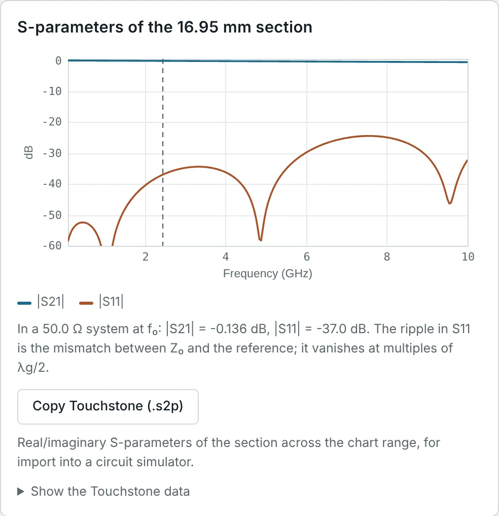
Return loss worse than simulated, ripple in S₁₁	Launch mismatch; two reflections beating (period Δf = v_p/2ℓ)	TDR to locate; tune pad and cutout
Narrow notches in S₂₁	Parallel-plate or cavity resonance; via-stub resonance	Add stitching vias; back-drill; add absorber in lids
Response shifted low in frequency	Dk higher than assumed; missing end corrections	Measure ε_eff with a ring; update the model
Loss higher than predicted	Rough copper, ENIG, solder mask, wrong tan δ	Two-line measurement; change finish or laminate
Poor isolation between lines	Coupling through shared pours, missing fences, lid cavity	Via fences, spacing ≥ 3h, cavity walls
Results vary board to board	Thickness and etch tolerance, glass weave	Controlled impedance spec; thicker substrate; spread-glass laminate

Worked Examples

Frequency Limits of Two Substrates

Problem: Find the transverse-resonance and TM₁ surface-wave limits for 50 Ω microstrip on 1.6 mm FR-4 (εr = 4.3, w = 3.07 mm) and 0.508 mm RO4003C (εr = 3.55, w = 1.14 mm).

FR-4

f_{T} = \frac{2.998 \times 10^{8}}{2.074 \times 7.42 \times 10^{- 3}} = 19.5 GHz

f_{T M_{1}} = \frac{2.998 \times 10^{8} \times 1.342}{\sqrt{2} π \times 1.6 \times 10^{- 3} \times 1.817} = 31.2 GHz

RO4003C 0.508 mm

f_{T} = \frac{2.998 \times 10^{8}}{1.884 \times 2.68 \times 10^{- 3}} = 59.4 GHz

f_{T M_{1}} = \frac{2.998 \times 10^{8} \times 1.297}{\sqrt{2} π \times 0.508 \times 10^{- 3} \times 1.597} = 108 GHz

Answer: FR-4 1.6 mm: keep below ≈ 10 GHz; RO4003C 0.508 mm: usable to ≈ 30 GHz

In practice the FR-4 board hits a loss limit (0.33 dB/cm at 10 GHz, Part 9) and a discontinuity limit (Part 13) long before its mode limit; the thin RO4003C board is limited by connectors and launches first.

Impedance Tolerance from Etch and Thickness

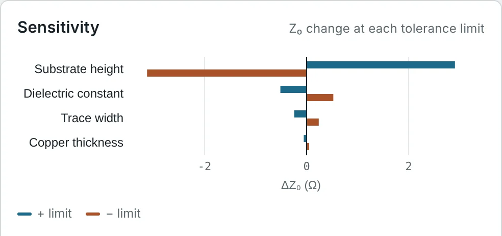
Problem: A 50 Ω microstrip on 0.508 mm RO4003C (w = 1.137 mm) is built with width tolerance ±0.025 mm and thickness tolerance ±0.038 mm. Find the Z₀ spread.

Hammerstad–Jensen at each limit

w \pm 0.025 : 50.7 / 49.3 Ω h \pm 0.038 : 47.6 / 52.3 Ω

Root-sum-square of independent errors

Δ Z_{0} \approx \sqrt{{0.69}^{2} + {2.35}^{2}} = 2.4 Ω (\pm 4.9 %)

Answer: about ±2.4 Ω (±5%), dominated by the substrate thickness

The ±0.038 mm thickness tolerance is 7.5% of a 0.508 mm board, against 2% for the width. A ±5% controlled-impedance specification is achievable only if the fabricator adjusts the width for the measured laminate thickness — which is exactly what the specification asks them to do.

Excess Capacitance of a Connector Pad

Problem: An edge-launch SMA pin lands on a 1.6 mm × 2.5 mm pad at the end of the 1.14 mm, 50 Ω line on 0.508 mm RO4003C. Estimate the pad's excess capacitance and its reflection at 10 and 20 GHz. What happens if the ground is cut away under the pad, so that it references a plane 1.016 mm below?

Pad as a short low-impedance line (Z_p = 40.0 Ω, ε_eff = 2.87)

τ = \frac{2.5 \times 10^{- 3} \sqrt{2.87}}{c} = 14.1 ps

C_{ex} = τ (\frac{1}{Z_{p}} - \frac{Z_{p}}{Z_{0}^{2}}) = 0.128 pF

Shunt-C reflection, x = ωC_exZ₀

10 GHz : x = 0.40, | Γ | = 0.20 (14.1 dB)

20 GHz : x = 0.80, | Γ | = 0.37 (8.6 dB)

With the cutout (Z_p = 61.6 Ω)

C_{ex} = - 0.115 pF (now inductive — over-compensated)

Answer: 0.13 pF excess — return loss only 14 dB at 10 GHz; a full cutout over-corrects

The correct cutout lies between the two: removing ground under part of the pad, or under the whole pad with a narrower pad, tuned in a 3D simulation with the connector model. Done well, launches on this board reach 20 dB return loss to beyond 20 GHz.

Via-Fence Pitch at 20 GHz

Problem: A GCPW on RO4003C must work to 20 GHz. Choose a via-fence pitch, taking the wavelength in the dielectric as the worst case.

Wavelength in the dielectric

λ_{d} = \frac{c}{f \sqrt{ε_{r}}} = \frac{14.99}{1.884} = 7.96 mm

\frac{λ_{d}}{10} = 0.80 mm

\frac{λ_{d}}{20} = 0.40 mm

Answer: pitch 0.4–0.8 mm; with 0.3 mm drills, about 0.6 mm is a practical choice

The fence also needs vias close to the slot edge (within about one substrate height) so the GCPW's ground is defined by the vias rather than by the far edge of the pour.

Cavity Resonance of an Unstitched Ground Pour

Problem: A 50 mm × 30 mm top-layer ground pour on 0.508 mm RO4003C is tied to the bottom plane only at a few points near its edges. Find the lowest parallel-plate resonances, and the resonance of a channel between two via rows 2.0 mm apart.

Rectangular cavity, f_mn = (c/2√εr)√((m/a)² + (n/b)²)

f_{10} = \frac{2.998 \times 10^{8}}{2 \times 1.884 \times 0.050} = 1.59 GHz

f_{01} = 2.65 GHz

f_{11} = 3.09 GHz

Channel between via rows

f_{c} = \frac{c}{2 a \sqrt{ε_{r}}} = \frac{2.998 \times 10^{8}}{2 \times 2.0 \times 10^{- 3} \times 1.884} = 39.8 GHz

Answer: pour resonances from 1.6 GHz — right in the operating band; the 2 mm via channel is safe to ≈ 40 GHz

Stitching the pour with vias at the fence pitch of Example 4 splits the cavity into regions too small to resonate below the highest operating frequency.

Locating Mismatches from S₁₁ Ripple

Problem: A test board on RO4003C (ε_eff ≈ 2.79) shows S₁₁ ripple with a period of 1.6 GHz. How far apart are the two dominant reflections?

Reflections a distance ℓ apart repeat in phase every Δf = v_p/2ℓ

v_{p} = \frac{c}{\sqrt{2.79}} = 1.795 \times 10^{8} m/s

ℓ = \frac{v_{p}}{2 Δ f} = \frac{1.795 \times 10^{8}}{3.2 \times 10^{9}} = 56 mm

Answer: 56 mm — the length of the board between its two connectors

The ripple is the two launches beating against each other. Improving either launch reduces the ripple amplitude; TDR (Example 10) confirms which one is worse.

Designing a TRL Calibration Line

Problem: Design the TRL line standard for 2–16 GHz on 0.508 mm RO4003C, taking ε_eff ≈ 2.85 at 9 GHz (dispersion included).

90° at the band centre f_m = 9 GHz

Δ ℓ = \frac{c}{4 f_{m} \sqrt{ε_{eff}}} = \frac{299.79}{4 \times 9 \times 1.688} = 4.93 mm

Phase at the band edges

ϕ (2 GHz) = 90^{\circ} \times \frac{2}{9} = 20^{\circ}

ϕ (16 GHz) = 90^{\circ} \times \frac{16}{9} = 160^{\circ}

Answer: a line 4.93 mm longer than the thru covers exactly 2–16 GHz

Below 2 GHz a second, longer line (or a load standard) is needed. The reflect standard is an open or a short of the same launch, and the thru defines the reference plane at its centre.

Measuring Line Loss with Two Lines

Problem: Two 50 Ω microstrip lines on 0.813 mm RO4003C, 25 mm and 75 mm long with identical launches, measure 0.52 dB and 0.87 dB insertion loss at 10 GHz (after allowing for their small mismatch). Find α and the loss of each connector.

The connectors cancel in the difference

α = \frac{0.87 - 0.52}{5.0 cm} = 0.070 dB/cm

{IL}_{conn} \approx \frac{0.52 - 2.5 \times 0.070}{2} = 0.17 dB

Answer: α = 0.070 dB/cm — 11% above the 0.063 dB/cm predicted for smooth copper (Part 9); 0.17 dB per launch

The excess is typical of copper roughness and surface finish. The measured α can now be used to calibrate the roughness model in the simulator.

Feed-Line Loss and Receiver Noise Figure

Problem: An 80 mm microstrip feed between a 2.45 GHz antenna and an LNA is built either on 1.6 mm FR-4 (α ≈ 0.080 dB/cm) or on 0.813 mm RO4003C (α ≈ 0.021 dB/cm). How much does the choice change the receiver noise figure?

Loss before the LNA adds directly to the noise figure

FR-4 : 8 \times 0.080 = 0.64 dB

RO4003C : 8 \times 0.021 = 0.17 dB

Δ NF \approx 0.47 dB

Answer: about 0.5 dB better noise figure on RO4003C

Half a decibel of noise figure is worth about 6% more range in free space (Friis equation). The cheaper alternative is to move the LNA close to the antenna and keep the FR-4 — the loss then comes after the gain, where it hardly matters (working in dB).

Reading a TDR Trace

Problem: A TDR with 35 ps rise time shows a dip to ρ = −0.05 at 0.42 ns after the launch on a RO4003C line (v_p = 1.795 × 10⁸ m/s). Where is the discontinuity, what is the local impedance, and what is the spatial resolution?

Location and impedance

d = \frac{v_{p} t}{2} = \frac{1.795 \times 10^{8} \times 0.42 \times 10^{- 9}}{2} = 37.7 mm

Z = 50 \frac{1 + ρ}{1 - ρ} = 45.2 Ω

Resolution

Δ x \approx \frac{v_{p} t_{r}}{2} = \frac{1.795 \times 10^{8} \times 35 \times 10^{- 12}}{2} = 3.1 mm

Answer: a capacitive discontinuity 37.7 mm from the launch, locally 45 Ω

A dip means excess capacitance — for example a component pad, a wide bend or a via pad. Features shorter than about 3 mm are blurred, so the true impedance of a small pad is lower than the 45 Ω the trace suggests.

Summary

Choose the structure for the job: microstrip for general use, GCPW for launches and isolation, stripline for buried routing.
Choose the substrate for loss, Dk stability and thickness tolerance; check the frequency limits f_T and f_TM₁.
Calculate dimensions, confirm them in a 2D solver with mask and etch, and specify controlled impedance.
Design launches with ground cutouts and nearby ground vias; stitch pours and fence RF lines at ≤ λ_g/10 pitch.
Simulate critical regions in 2.5D or 3D with proper ports, materials, convergence and de-embedding.
Verify with VNA (SOLT or TRL), two-line loss and TDR — and feed the results back into the models.

This completes the Transmission Lines & Microwave Circuits series. The series overview lists all fifteen parts; the Smith Chart series develops matching networks for these lines, and the Antenna Fundamentals series follows the signal off the board and into space.

📘 Go deeper: Impedance matching for real lines

Use the Smith chart to design matching networks with lines and stubs on the substrates chosen here. Open Impedance Matching Using the Smith Chart →

Put It Into Practice

Use the NEXT ANTENNAS calculators to apply the ideas from this article to real lines and circuits.

Transmission Lines Microstrip & Stripline Impedance Calculator Field-solver backed design of microstrip, embedded microstrip, stripline, GCPW and differential pairs: width, εeff, Z₀, loss, dispersion and tolerance. Open calculator → Link & Power VSWR & Return Loss Calculator Convert between VSWR, return loss, reflection coefficient and mismatch loss. Open calculator → Impedance Matching Smith Chart Visualiser Plot impedances, move along lines and stubs, load Touchstone files and design matching networks. Open calculator → All Tools All RF Calculators Browse every NEXT ANTENNAS calculator for RF, microwave and antenna design. Open calculator →