Introduction to Stripline Transmission Lines
Microstrip (Part 9) and CPW (Part 10) are open on top: their fields extend into the air, so they radiate a little, couple to neighbouring lines and to the enclosure lid, and are slightly dispersive. In a multilayer board there is a natural way to avoid all three: bury the strip between two ground planes. This is stripline, first used by Barrett in the early 1950s as a "flat coax", and still the standard line for the inner layers of RF and high-speed digital boards.
This article treats stripline first, then returns to grounded coplanar waveguide, the surface-layer line that achieves much of stripline's isolation while keeping components accessible. The two, with microstrip, are the building blocks of every modern multilayer RF board.
Stripline Structure and Geometry
A symmetric stripline is a flat strip of width W and thickness t, centred between two ground planes a distance b apart, in a homogeneous dielectric of permittivity εr (Fig 1). In a PCB, one ground is a layer above and the other a layer below, the dielectric being core and prepreg laminated together. The two grounds must be tied together frequently with vias; otherwise they can carry a parallel-plate mode between them.
Electric and Magnetic Field Distribution
The electric field runs from the strip to both ground planes — half upwards, half downwards — and fringes around the strip edges. The magnetic field circles the strip. Because the whole field is in one homogeneous dielectric, the boundary-condition argument of Part 9 that forced microstrip to be quasi-TEM does not apply: stripline carries a pure TEM wave, with
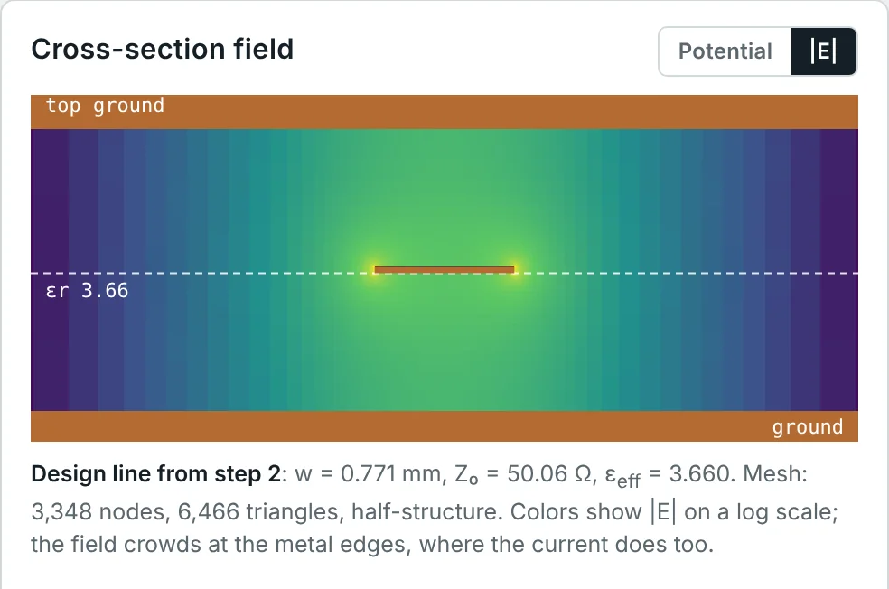
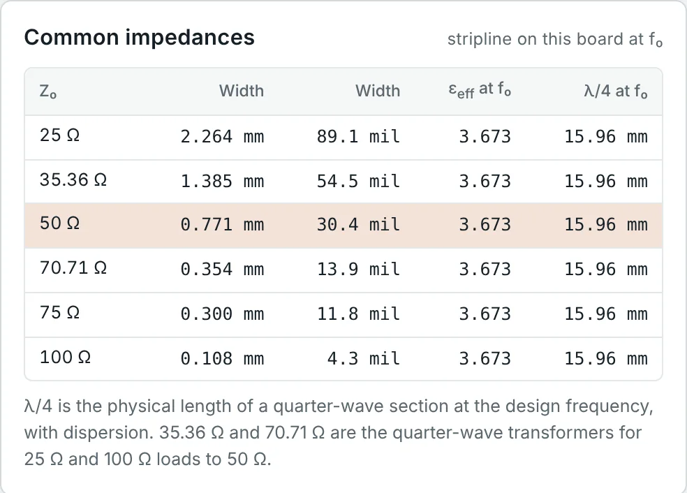
Three useful consequences follow: no dispersion (the electrical length is exactly proportional to frequency), no radiation from the line itself, and very low coupling to other lines beyond about one b away. Fig 2 shows the field of a 50 Ω stripline from the calculator's field solver.
Characteristic Impedance of Stripline
For a strip of zero thickness, stripline is one of the few planar lines with an exact closed-form impedance.
By symmetry, the strip sees two identical half-regions, above and below. A conformal mapping transforms each half — strip to ground plane — into a parallel-plate capacitor whose width-to-spacing ratio is K(k)/K(k′), with a modulus determined by W/b:
(the factor 4 counts the two halves and the two edges of each). Since the line is TEM, Z₀ = √εr/(cC):
For hand calculation, Pozar's fit to this result (accuracy about 1%) is simpler:
Strip thickness lowers Z₀, because the strip's side walls add capacitance and the strip occupies part of the space between the grounds. For 35 µm copper in b = 1.524 mm the calculator's field solver needs W = 0.771 mm for 50 Ω, versus 0.833 mm from the exact zero-thickness formula — a 7% correction, larger than in microstrip because the field is squeezed from both sides.
Stripline Design Parameters
- Ground spacing b. Z₀ depends on W/b, so b sets the strip width for a given impedance. In a stack-up, b is the total dielectric between the two reference planes (core plus prepreg plus the strip thickness).
- Strip width. For the same dielectric thickness to the nearest ground, a stripline is roughly half as wide as a microstrip, because it has a ground on both sides. Narrower strips mean higher conductor loss.
- Dielectric. Since εeff = εr, a stripline has all of its field in the dielectric and its dielectric loss is higher than that of a microstrip on the same laminate (Example 6). Stripline therefore benefits even more from a low-loss material.
- Higher-order modes. The first higher-order (TE) mode can propagate when the strip plus its fringing region becomes half a wavelength wide. Pozar gives its cutoff as
Symmetric and Asymmetric Stripline
In a real stack-up the strip is rarely exactly in the middle: it sits on a core and is covered by prepreg of a different thickness, or two signal layers share the space between a pair of planes (dual stripline). In this asymmetric or offset stripline the strip is a distance h₁ from one ground and h₂ from the other.
The capacitance from the strip to the near ground and to the far ground act in parallel. Each is approximately that of half of a symmetric stripline with ground spacing 2h₁ or 2h₂. Since Z₀ ∝ 1/C for a TEM line of fixed εr, the impedances combine like parallel resistances:
Asymmetry has two effects. The impedance is dominated by the nearer ground, so the strip can be made narrower for a given Z₀; and the return current divides unequally between the two planes — mostly in the nearer one — which matters for via placement and for any gap or split in that plane. If the strip is much closer to one plane, the line behaves almost like an embedded microstrip.
Introduction to Grounded Coplanar Waveguides
Part 10 introduced grounded CPW as CPW with a ground plane underneath. On PCBs it is often the best of both worlds: like microstrip it uses the board's ground layer, so it works on standard two-layer and multilayer boards; like CPW it has ground right next to the strip, so shunt components connect directly and adjacent lines are isolated by a strip of ground between them. Its field is partly coplanar (into the slots) and partly microstrip-like (down to the bottom ground), and the balance is set by the gap: narrow gaps make it CPW-like, wide gaps microstrip-like (the table in Part 10).
GCPW Structure and Grounding
A GCPW has three ground conductors — two top grounds and the bottom ground — and only works as intended if all three stay at the same potential along the line. Without connections between them, the structure supports unwanted modes:
- Parallel-plate (patch) modes between each top ground and the bottom ground, which resonate at frequencies set by the size of the ground areas (Example 9 of Part 10).
- Slot-line and coupled-slot modes when the two top grounds are at different potentials.
- Microstrip-like leakage where the top grounds end or are interrupted, letting the field spread under them.
All three are suppressed by connecting the top grounds to the bottom ground with rows of plated vias — via fences — along both sides of the line.
Via Fences and Ground Connections
A row of vias acts as a wall for the fields only if the gaps between vias are much shorter than a wavelength. Practical rules, widely used in RF PCB design:
| Rule | Typical value | Reason |
|---|---|---|
| Via pitch along the line | ≤ λg/10, preferably λg/20 at the highest frequency | Keeps the gaps between vias electrically small, so no field leaks and no resonance fits between vias |
| Distance from via to slot edge | About s to 2s (and ≥ 1–2 via diameters) | Ties the ground down where the return current flows |
| Top-ground width | ≥ w + 2s on each side | Keeps the impedance close to the infinite-ground value |
| Extra vias | At bends, junctions, component grounds and line ends | Discontinuities excite the unwanted modes |
| Stripline fences | Both sides of the strip, ≤ λg/10, at about b to 2b from the strip | Suppress the parallel-plate mode between the two grounds |
Each via has inductance, which is why a single via is a poor ground at microwave frequencies and why component grounds use several vias in parallel. A useful estimate for a via of length h and diameter d is
Stripline vs. Microstrip vs. GCPW
| Property | Microstrip | Stripline | GCPW |
|---|---|---|---|
| Mode | Quasi-TEM | Pure TEM | Quasi-TEM |
| εeff | (εr + 1)/2 to εr, frequency dependent | εr exactly | Between microstrip and CPW values |
| Dispersion | Moderate | None | Low |
| Radiation / coupling | Highest | Lowest | Low (with via fences) |
| Width for 50 Ω (RO4350B, 0.76 mm to ground) | ≈ 1.6 mm | ≈ 0.77 mm | Adjustable with the gap |
| Component access | Direct | Through vias | Direct, with grounds alongside |
| Dielectric loss | Lower (part of the field in air) | Higher (all in dielectric) | Intermediate |
| Conductor loss | Lowest for a given h | Higher (narrower strip) | Higher with narrow gaps |
| Board layers needed | 2 | 3+ (signal between two planes) | 2 |
| Typical use | General RF, antennas | Inner-layer routing, filters, couplers, high-speed digital | mm-wave, connector launches, dense RF layouts |
Differential Pairs on Multilayer Boards
High-speed digital interfaces and many RF ICs use differential pairs: two coupled lines carrying equal and opposite signals. Part 4 introduced the two impedances that describe them — the odd-mode impedance Z₀ₒ (for the differential signal) and the even-mode impedance Z₀ₑ (for common-mode noise) — and the specified values Zdiff = 2Z₀ₒ and Zcomm = Z₀ₑ/2. Fig 4 shows a 100 Ω differential microstrip pair on 0.813 mm RO4003C from the calculator: each line is 1.048 mm wide with a 0.410 mm gap, Z₀ₒ = 50.0 Ω and Z₀ₑ = 81.3 Ω.
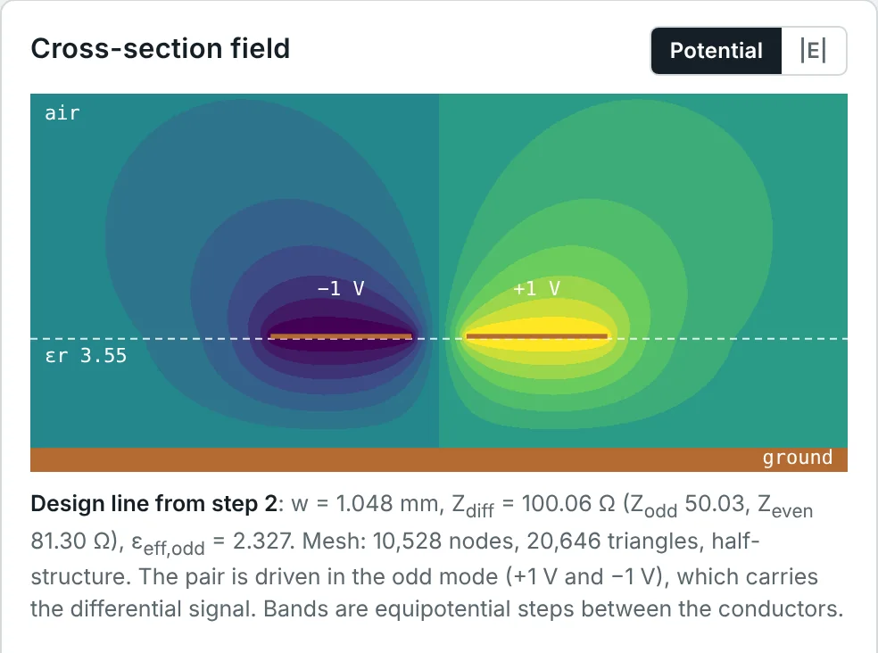
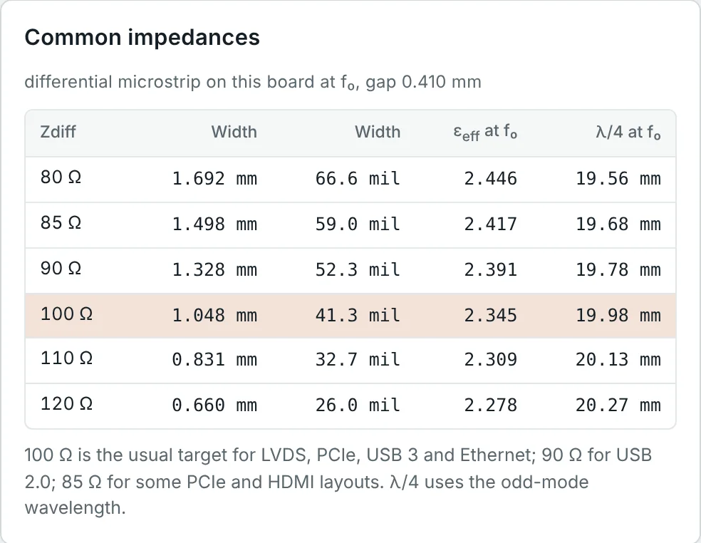
In the odd mode the plane of symmetry between the lines is a virtual ground (an electric wall), so each line sees extra capacitance to its neighbour and Z₀ₒ is lower than the isolated-line impedance; in the even mode it is a magnetic wall and Z₀ₑ is higher. The calculator solves the cross-section twice, once with each wall, to obtain both. Differential stripline works the same way, with εeff = εr for both modes; differential microstrip has different εeff for the two modes (2.33 and 2.82 here), so its odd and even modes travel at slightly different speeds — a source of mode conversion that stripline avoids.
Applications in Multilayer RF PCBs
A typical four-layer RF board puts GCPW or microstrip on layer 1 for components and connectors, a solid ground on layer 2 as their reference, stripline or power on layer 3, and ground on layer 4. More complex radios and phased arrays use eight to twenty layers, with several stripline layers for feed networks and digital control, each sandwiched between ground planes. Five practical rules make such boards work:
- Every RF line needs a continuous reference plane directly next to it. A gap or split in the plane under a trace forces the return current around it and creates a large discontinuity.
- Design the impedance from the real stack-up: the dielectric thickness to the nearest planes, the actual εr of core and prepreg (often different), and the finished copper thickness.
- Tie the planes together with vias along every RF line and around the board edge (via fences and stitching).
- Treat layer transitions as discontinuities. A signal via from a surface GCPW to an inner stripline is a short coaxial section; ground vias must surround it closely to carry the return current between the planes. Such transitions are designed and simulated as components (Part 13).
- Use stripline for long, sensitive or densely packed routes, and the surface layer for components and short connections.
Worked Examples
The examples use c = 299.79 mm/ns and K(k)/K(k′) from Hilberg's approximations (Part 10).
50 Ω Stripline Width by the Synthesis Formula
Problem: Design a 50 Ω stripline in RO4350B (εr = 3.66) with ground-plane spacing b = 1.524 mm, neglecting strip thickness.
The field solver, with 35 µm copper, gives 0.771 mm — the strip thickness reduces the width by 7%. On a board this size the difference is about 60 µm, comparable to the etch tolerance, so it must be included.
Checking with the Exact Conformal-Mapping Formula
Problem: Find the exact zero-thickness impedance of W = 0.829 mm, b = 1.524 mm in RO4350B.
The exact formula needs W = 0.833 mm for exactly 50.0 Ω. For zero-thickness strips, either formula is adequate; thickness is the larger correction in practice.
Quarter-Wave Length in Stripline
Problem: Find the length of a quarter-wave section at 5.8 GHz in RO4350B stripline, for any impedance.
This is the practical advantage visible in Fig 2b: in stripline a 35 Ω and a 70 Ω quarter-wave section have exactly the same length, unlike in microstrip where they differ by several per cent. Coupled-line filters and couplers designed in stripline therefore need no correction for unequal phase velocities.
Upper Frequency Limit of a Stripline
Problem: Find the first higher-order-mode cutoff for the 50 Ω stripline (W = 0.771 mm, b = 1.524 mm, εr = 3.66).
Thinner dielectrics push the limit up in proportion: the same impedance in a stack with b = 0.5 mm works to about 120 GHz. Via fences beside the strip keep the parallel-plate mode from coupling to the line well before this limit.
Impedance of an Offset Stripline
Problem: A 0.25 mm strip in RO4350B is 0.2 mm from one ground and 0.4 mm from the other. Estimate Z₀ with the parallel-combination rule.
The nearer ground (Z₀(0.4) = 46 Ω) dominates. The same strip centred between grounds 0.6 mm apart would have 57.8 Ω; the offset version is lower because the near ground dominates, and it carries about 60% of its return current in the nearer plane.
Dielectric Loss: Stripline vs Microstrip
Problem: Compare the dielectric attenuation at 10 GHz of a 50 Ω stripline in RO4350B (tan δ = 0.0037) with a 50 Ω microstrip on 0.762 mm RO4350B (εeff = 2.82).
All of the stripline's field is in the dielectric, so its dielectric loss is about 28% higher. Its conductor loss is also higher (narrower strip). The price of stripline's isolation is loss — so long RF stripline runs use the lowest-loss laminate available.
Via-Fence Pitch for a 10 GHz Stripline
Problem: Choose the via pitch for fences along a RO4350B stripline operating up to 10 GHz.
With 0.3 mm drills, a 0.8 mm pitch is easy to manufacture. Place the fences about b to 2b from the strip edge so that they do not change its impedance.
Odd- and Even-Mode Impedances of a 100 Ω Pair
Problem: The calculator's 100 Ω differential microstrip on RO4003C has Z₀ₒ = 50.0 Ω and Z₀ₑ = 81.3 Ω. Find Zdiff, Zcomm and the coupling coefficient.
The same coupled-line parameters describe a −12.5 dB directional coupler — coupled lines are both a differential interconnect and a microwave component (Part 14 uses them in filters). Moving the lines apart lowers C, raises Z₀ₒ, and would need wider lines to keep 100 Ω.
Why One Ground Via Is Not Enough
Problem: Estimate the inductance and reactance at 10 GHz of a 0.3 mm via through a 1.524 mm board. How many vias in parallel bring the reactance below 10 Ω (ignoring mutual coupling)?
In practice mutual inductance between closely spaced vias reduces the benefit, so even more are used, spread apart. This is why GCPW, with its ground right beside the component, is preferred at high frequencies over microstrip with via grounds.
Choosing Lines for a Four-Layer RF Board
Problem: A four-layer RO4350B board has 0.762 mm between each signal layer and its nearest plane. Compare the 50 Ω widths of a surface microstrip (L1 referenced to L2) and of a centred stripline between L2 and L4 (b = 1.524 mm), and their quarter-wave lengths at 5.8 GHz.
The stripline is half as wide and 12% shorter for the same electrical length, so inner-layer filters and couplers are more compact — at the cost of higher loss and of vias to reach them.
Summary
- Stripline: a strip between two grounds in one dielectric — pure TEM, εeff = εr, no dispersion, no radiation.
- Exact Z₀ (t = 0): (30π/√εr) K(k)/K(k′), k = sech(πW/2b); Pozar's fit W/b = 30π/(√εr Z₀) − 0.441. Thickness lowers Z₀ noticeably.
- Offset stripline ≈ parallel combination of two symmetric striplines with spacings 2h₁ and 2h₂.
- Grounded CPW combines microstrip's back ground with CPW's coplanar grounds; via fences at ≤ λg/10 are essential.
- Stripline has the best isolation but the highest loss and needs vias; microstrip is simplest; GCPW suits mm-wave and dense layouts.
- Differential pairs are specified by Zdiff = 2Z₀ₒ and Zcomm = Z₀ₑ/2.
Stage 3 is complete. Stage 4 uses lines of chosen electrical length as circuit elements: Part 12: Quarter-Wave and Half-Wave Lines and Stubs covers quarter-wave transformers, half-wave lines and open and short stubs.
The stubs and transformers of the next part are drawn in whichever of these three lines the board uses. Open Smith Chart & Impedance Matching series →
Put It Into Practice
Use the NEXT ANTENNAS calculators to apply the ideas from this article to real lines and circuits.