Transmission Line Losses Explained

Fig 1 — Attenuation against frequency for RG-58 coax (smooth-copper model, PE dielectric) and 50 Ω microstrip on 1.6 mm FR-4: conductor loss rises as √f, dielectric loss as f. On FR-4 the dielectric dominates above about 20 MHz; on PE coax, conductor loss dominates to well above 10 GHz

RG-58 conductorRG-58 dielectricRG-58 totalFR-4 microstrip conductorFR-4 microstrip dielectricFR-4 microstrip total

Introduction to Transmission-Line Losses

Every real line loses some of the power it carries. In a receiver the loss adds directly to the noise figure; in a transmitter it is heat in the cable and power that never reaches the antenna; on a high-speed board it closes the eye of the data signal. Part 3 represented loss by two circuit elements — series resistance R′ and shunt conductance G′ — and Part 5 showed that for a low-loss line they add up to the attenuation constant α = R′/2Z₀ + G′Z₀/2.

This article opens those two elements up. Three physical mechanisms remove power from a guided wave:

Conductor loss α_cOhmic heating of the metal, concentrated in a thin skin at RF and increased by surface roughness. Grows roughly as √f.

Dielectric loss α_dHeating of the insulator as its molecules follow the alternating field, set by the loss tangent. Grows as f.

Radiation loss α_rPower that leaves open lines (microstrip, CPW, two-wire) as radiation, mostly at bends and discontinuities. Grows rapidly with f and substrate thickness.

Derivation — attenuation from power loss

A wave carries power P(z) = P₀e^−2αz, so the power lost per metre is −dP/dz = 2αP. Turning this round gives a general recipe, the perturbation method: calculate the fields of the lossless line, compute the power they dissipate per metre, P′_loss, and divide:

Attenuation from dissipated power

α = \frac{P_{loss}^{'}}{2 P} α = α_{c} + α_{d} + α_{r}

For the conductor, P′_loss = ½|I|²R′ and P = ½|I|²Z₀, giving α_c = R′/2Z₀; for the dielectric, P′_loss = ½|V|²G′ and P = ½|V|²/Z₀, giving α_d = G′Z₀/2.

Conductor Losses

At DC the current spreads uniformly over each conductor's cross-section, and R′ is simply the resistivity divided by the area. At radio frequencies the current crowds into a thin layer at the conductor surfaces that face the other conductor — the skin effect — and the effective area, and therefore R′, depends on frequency.

Skin Effect

Derivation — skin depth and surface impedance

Inside a good conductor (σ ≫ ωε) the displacement current is negligible, and Maxwell's equations reduce to a diffusion equation for the current density J flowing parallel to the surface, at depth x below it:

\frac{d^{2} J}{d x^{2}} = j ω μ σ J \Rightarrow J (x) = J_{0} e^{- (1 + j) x / δ_{s}},

δ_{s} = \sqrt{\frac{2}{ω μ σ}} = \frac{1}{\sqrt{π f μ σ}}

The current decays exponentially, falling to 1/e at the skin depth δ_s, and its phase lags with depth. Integrating over the depth gives the total current per unit width, and dividing the surface electric field by it gives the surface impedance of the conductor:

Surface impedance

Z_{s} = \frac{1 + j}{σ δ_{s}} = R_{s} (1 + j)

R_{s} = \frac{1}{σ δ_{s}} = \sqrt{\frac{π f μ}{σ}}

R_s is the resistance of one square of conductor surface, as if the current flowed uniformly in a layer one skin depth thick. The equal reactive part is the internal inductance, which vanishes as δ_s → 0.

Fig 2 — Current density against depth below a copper surface: at 1 GHz (δ_s = 2.09 µm) and 10 GHz (δ_s = 0.66 µm), 99% of the current flows within 5δ_s

1 GHz10 GHz

The skin depth in copper is 8.5 mm at 60 Hz, 66 µm at 1 MHz, 2.1 µm at 1 GHz and 0.66 µm at 10 GHz. Since standard PCB copper is 17–35 µm thick and cable conductors much thicker, at RF all conductors are "thick" and the current flows only in their surfaces. Two practical consequences follow:

R′ ∝ √f. For coax, R′ = (R_s/2π)(1/a + 1/b), and α_c = R′/(2Z₀) grows as √f. Doubling the frequency increases conductor loss by 41%.
Only the surface matters. Silver plating (σ 6% higher than copper) and smooth surfaces reduce loss; a thin layer of poor conductor on the surface — nickel under gold in ENIG finishes, oxide, or tin — can increase it noticeably, because the current has to flow through it.

Conductor loss of common lines

Conductor attenuation (smooth conductors)

α_{c, coax} = \frac{R_{s}}{4 π Z_{0}} (\frac{1}{a} + \frac{1}{b})

α_{c, microstrip} \approx \frac{R_{s}}{Z_{0} w}

Coax: exact for the TEM mode. Microstrip: first-order parallel-plate estimate (Part 9), within about ±30% for 50 Ω lines; Wheeler's incremental-inductance rule gives accurate values for any geometry.

Both formulas show the same design rule: bigger conductors have lower loss. For a fixed Z₀, scaling a coax up by a factor k reduces α_c by k; widening a microstrip (on a thicker substrate, to keep Z₀) does the same. That is why low-loss feeders are thick, and why loss on thin, narrow PCB traces rises quickly.

Surface Roughness Effects

Copper foil for PCBs is deliberately roughened so that it bonds to the laminate. Once the skin depth becomes comparable to the height of the surface teeth, the current has to follow the profile up and down, travelling a longer path through a smaller effective cross-section, and the loss rises. The classic model, due to Hammerstad, multiplies the smooth-conductor loss by a factor K_r:

Hammerstad roughness factor

K_{r} = 1 + \frac{2}{π} \tan^{- 1} [1.4 {(\frac{Δ_{rms}}{δ_{s}})}^{2}]

α_{c} = K_{r} α_{c, smooth}

Δ_rms is the rms surface roughness. K_r → 1 for a smooth surface and saturates at 2 when the roughness is several skin depths — the current path is then roughly twice as long.

Fig 3 — Hammerstad roughness factor against Δ_rms/δ_s. Marked: standard ED copper (Δ ≈ 1.5 µm) at 1 GHz and 10 GHz

K_r

Laminate suppliers therefore offer several copper grades: standard electrodeposited (ED) copper with Δ_rms of 1.5–3 µm, reverse-treated (RTF) and very-low-profile (VLP, HVLP) foils at 0.4–1 µm, and rolled annealed copper below 0.5 µm. Above about 10 GHz the choice of foil can change conductor loss by 50%. At very high frequencies, or with very rough foils, the Hammerstad model underestimates the loss because it saturates at 2; more detailed models (such as Huray's "snowball" model) are then used.

Dielectric Losses

A dielectric stores energy because its molecules and atoms polarise in an applied field. In an alternating field the polarisation lags slightly behind the field, and some energy is converted to heat each cycle. This is described by a complex permittivity:

Complex permittivity

ε = ε^{'} - j ε^{″} = ε_{0} ε_{r} (1 - j \tan δ)

\tan δ = \frac{ε^{″}}{ε^{'}}

Loss Tangent

The loss tangent tan δ is the ratio of the lossy to the lossless part of the permittivity — equivalently, the ratio of the conduction-like current to the displacement current in the dielectric. It is the single number that characterises a material's dielectric loss, and it varies over three orders of magnitude between materials:

Material	εr	tan δ (≈ 1–10 GHz)	Dielectric loss of a 50 Ω line at 10 GHz
Air, foam PE	1.0–1.5	< 0.0001	negligible
PTFE (RT/duroid 5880)	2.1–2.2	0.0002–0.0009	≈ 0.03–0.1 dB/cm
Polyethylene	2.25	0.0002–0.0004	≈ 0.03 dB/cm
Rogers RO4003C	3.55	0.0027	≈ 0.04 dB/cm (microstrip)
Alumina 99.6%	9.8	0.0001	≈ 0.003 dB/cm
FR-4	4.2–4.6	0.015–0.025	≈ 0.3 dB/cm (microstrip)

Derivation — dielectric attenuation

From Part 3, G′ = ωC′ tan δ. Substituting into α_d = G′Z₀/2 and using Z₀ = 1/(v_pC′):

Dielectric attenuation of a line filled with one dielectric

α_{d} = \frac{ω C^{'} \tan δ Z_{0}}{2} = \frac{ω \tan δ}{2 v_{p}} = \frac{β}{2} \tan δ = \frac{π \sqrt{ε_{r}}}{λ_{0}} \tan δ

Independent of the geometry: every coax or stripline in the same dielectric has the same α_d. For microstrip, replace tan δ by the effective loss tangent q εr tan δ/εeff (Part 9). Per guided wavelength, α_dλ_g = π tan δ nepers.

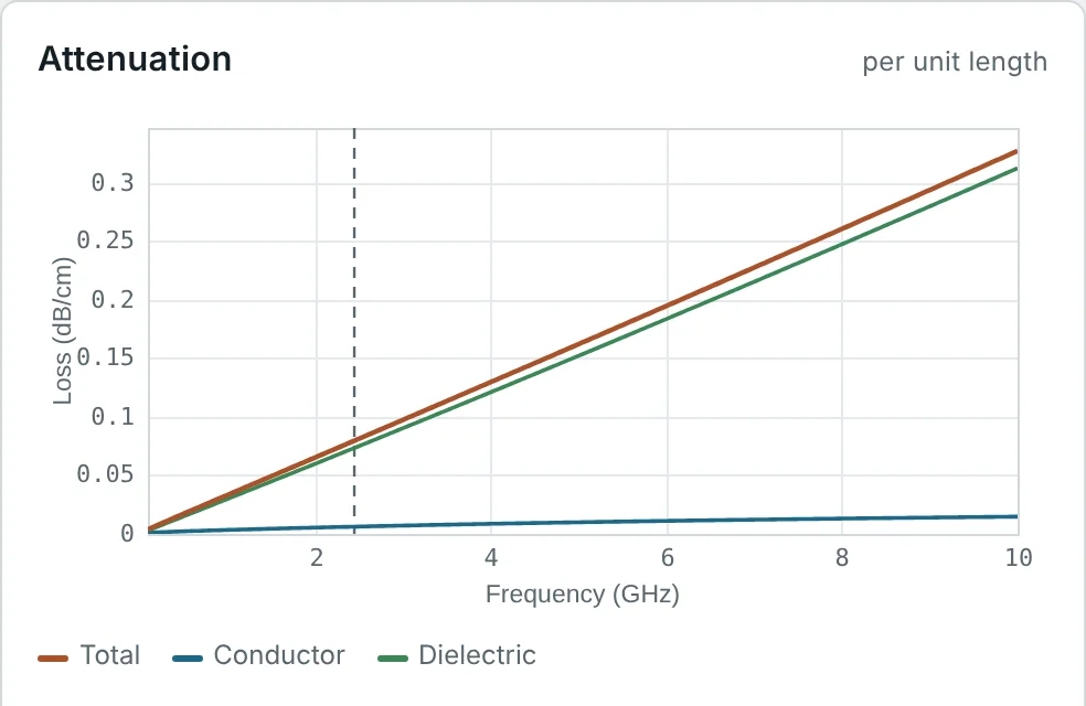
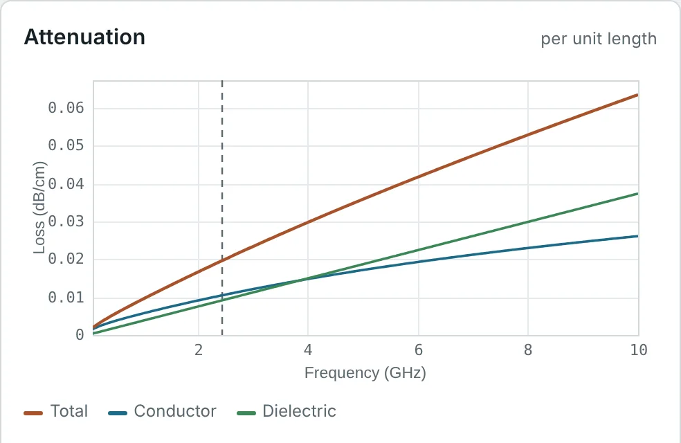
Because α_d ∝ f while α_c ∝ √f, dielectric loss always wins at a high enough frequency. Where the crossover lies depends on the material: on PE coax it is above 100 GHz, on FR-4 microstrip around 20 MHz (Fig 1). Real loss tangents also vary with frequency — FR-4's tan δ and εr both drift over a decade of frequency — which is why wideband models such as Djordjevic–Sarkar (used in the microstrip calculator) describe the material over the whole band rather than at a single point.

Attenuation of a 50 ohm FR-4 microstrip against frequency, almost entirely dielectric loss — Fig 4a — 50 Ω microstrip on 1.6 mm FR-4: dielectric loss is 92% of the total at 2.45 GHz. Try it in the Microstrip & Stripline Impedance Calculator →

Attenuation of a 50 ohm RO4003C microstrip with conductor and dielectric losses comparable — Fig 4b — The same impedance on 0.813 mm RO4003C: a quarter of the total loss, split evenly. Try it in the Microstrip & Stripline Impedance Calculator →

Radiation Losses

Closed lines — coax, stripline, waveguide — cannot radiate. Open lines can: some of their field extends into the surrounding space, and wherever the line's symmetry is broken, part of the guided wave is converted into a wave that travels away. On a straight, uniform microstrip radiation is very small; it arises mainly at discontinuities — open ends, bends, steps in width, T-junctions — and at the unbalanced currents on two-wire lines.

The radiated power from a microstrip discontinuity grows roughly as (h/λ₀)² — as the square of the substrate's electrical thickness — and decreases with higher εr, which holds the field more tightly. The open end of a narrow strip, for example, behaves like a small radiating slot with conductance of roughly

Radiation conductance of an open end of width w ≪ λ₀ (approximate)

G_{rad} \approx \frac{1}{90} {(\frac{w}{λ_{0}})}^{2} S

This is the same physics that makes a patch antenna radiate: its two open edges are wide (w ≈ λ/2) and its substrate thick, so the radiation conductance becomes large on purpose (antenna types).

Radiation loss is usually much smaller than conductor and dielectric loss in a well-designed circuit, but it causes other problems: coupling between parts of a circuit, unwanted emissions (EMC) and resonances in enclosures. It is minimised by using thin substrates at high frequencies, by shielding, and by choosing closed lines (stripline, GCPW with via fences, SIW) for sensitive circuits.

Attenuation Constant

The three contributions add in nepers per metre (and therefore in dB per metre):

Total attenuation

α = K_{r} α_{c} + α_{d} + α_{r} \approx K_{r} \frac{R^{'}}{2 Z_{0}} + \frac{G^{'} Z_{0}}{2} + α_{r}

Convert with α [dB/m] = 8.686 α [Np/m]. K_r is the roughness factor; α_r is usually treated through the discontinuities rather than per metre.

The attenuation also sets the quality factor of any resonator made from the line. For a resonant section with stored energy per metre W′ and power loss per metre 2αP, Q = ωW′/(2αP) = β/(2α), so a line with lower loss per wavelength makes a sharper filter (Part 14).

Insertion Loss

Insertion loss is the reduction in power delivered to a load when a component — here a length of line — is inserted between a matched source and load. For a matched line it is simply the attenuation times the length; in S-parameter terms it is −20 log|S₂₁|:

Insertion loss

IL = - 20 \log_{10} | S_{21} | = 8.686 α ℓ dB (matched line)

Mismatch at either end adds loss through reflection: approximately IL ≈ αℓ + ML_in + ML_out for small mismatches, where ML = −10 log(1 − |Γ|²).

Two distinctions matter in practice. First, insertion loss includes mismatch, but attenuation does not: a perfectly lossless line between mismatched terminations still has insertion loss. Second, loss and mismatch interact — a lossy line hides the mismatch at its far end, because the reflected wave is attenuated twice (Part 7). In a receiving system, the insertion loss L of a passive line also adds noise: its noise figure equals its loss, which is why a lossy feeder in front of a low-noise amplifier is so damaging.

Frequency Dependence of Transmission-Line Losses

Mechanism	Frequency dependence	Depends on	Dominant on
Conductor (smooth)	∝ √f	σ, conductor size, Z₀	Low-loss dielectrics, small conductors, low frequency
Roughness	K_r from 1 (low f) to 2 (high f)	Δ_rms/δ_s	PCB lines above a few GHz
Dielectric	∝ f (constant tan δ)	tan δ, εr — not geometry	Lossy laminates (FR-4) above tens of MHz; all lines at mm-wave
Radiation	∝ f² or faster at discontinuities	h/λ₀, εr, layout	Thick substrates, open lines, many discontinuities

On a log-log plot (Fig 1) the conductor and dielectric contributions are straight lines with slopes ½ and 1. Measuring a line's loss at two frequencies therefore separates them: fit α(f) = a√f + bf and the two coefficients give the conductor and dielectric parts. This is how signal-integrity engineers build loss models of PCB stack-ups from test-coupon measurements.

Methods to Reduce Transmission-Line Losses

Choose a low-loss dielectric. Above about 1 GHz, the laminate's tan δ is usually the biggest lever: RO4003C instead of FR-4 cuts dielectric loss by a factor of about eight.
Make conductors bigger. A larger coax or a wider trace on a thicker substrate (at the same Z₀) reduces conductor loss in proportion to its size.
Use smooth copper (VLP, HVLP, rolled) above a few GHz, and avoid lossy surface finishes on RF traces — immersion silver or OSP rather than ENIG at the highest frequencies.
Use air or foam dielectrics for cables and long runs — foam coax, air-dielectric hardline, waveguide.
Keep lines short. Put the low-noise amplifier at the antenna, and the radio close to it.
Avoid radiation with thin substrates at high frequencies, closed or shielded lines, and smooth transitions at discontinuities.
Match well. Mismatch adds to insertion loss and, through standing waves, raises the peak currents and the conductor loss.

Practical Loss Calculations

The examples use μ₀ = 4π × 10⁻⁷ H/m, σ_Cu = 5.8 × 10⁷ S/m and c = 2.998 × 10⁸ m/s.

Skin Depth in Copper and Aluminium

Problem: Calculate the skin depth in copper at 60 Hz, 1 MHz, 1 GHz and 10 GHz, and in aluminium (σ = 3.5 × 10⁷ S/m) at 1 GHz.

δ_s = 1/√(πfμ₀σ) — for copper δ_s = 66.1 µm/√(f [MHz])

60 Hz : 8.53 mm

1 MHz : 66.1 μ m

1 GHz : 2.09 μ m

10 GHz : 0.66 μ m

Aluminium at 1 GHz

δ_{s} = \frac{1}{\sqrt{π \times 10^{9} \times 4 π \times 10^{- 7} \times 3.5 \times 10^{7}}} = 2.69 μ m

Answer: 8.53 mm, 66 µm, 2.09 µm, 0.66 µm (Cu); 2.69 µm (Al at 1 GHz)

At 60 Hz the skin depth is comparable to large power conductors, which is why high-current busbars are flat. At RF it is microns: a 2 µm silver plating carries essentially all of the current at 10 GHz, and a hollow tube conducts as well as a solid rod.

Conductor Loss of RG-58 at 1 GHz

Problem: Estimate the conductor attenuation of RG-58 (a = 0.405 mm, b = 1.475 mm, Z₀ = 51.7 Ω) at 1 GHz, assuming smooth solid copper.

Surface resistance and R′

R_{s} = \sqrt{\frac{π \times 10^{9} \times 4 π \times 10^{- 7}}{5.8 \times 10^{7}}} = 8.25 m Ω

R^{'} = \frac{0.00825}{2 π} (\frac{1}{0.405} + \frac{1}{1.475}) \times 10^{3} = 4.13 Ω / m

Attenuation

α_{c} = \frac{4.13}{2 \times 51.7} = 0.040 Np/m = 0.347 dB/m = 34.7 dB/100 m

Answer: about 35 dB/100 m (smooth copper)

Real RG-58 is specified at about 60–65 dB/100 m at 1 GHz. The braid, the stranded centre conductor and the tin plating on some versions nearly double the ideal conductor loss — a reminder that the smooth-conductor formula is a lower bound.

Dielectric Loss of a PTFE Coax at 10 GHz

Problem: Find the dielectric attenuation of a PTFE-filled coax (εr = 2.1, tan δ = 2 × 10⁻⁴) at 10 GHz.

α_d = (β/2) tan δ

β = \frac{2 π \times 10^{10} \times \sqrt{2.1}}{2.998 \times 10^{8}} = 303.7 rad/m

α_{d} = \frac{303.7 \times 2 \times 10^{- 4}}{2} = 0.0304 Np/m = 0.26 dB/m

Answer: α_d ≈ 0.26 dB/m, the same for every PTFE coax at 10 GHz

The result does not depend on the cable size. Conductor loss of a 0.141″ semi-rigid cable at 10 GHz is three to four times larger, so even with PTFE the conductors dominate in small coax; in large air-line or foam cables the dielectric share grows.

Where Dielectric Loss Overtakes Conductor Loss on FR-4

Problem: On the 50 Ω FR-4 microstrip of Part 9, the calculator gives α_c = 0.0062 dB/cm and α_d = 0.0734 dB/cm at 2.45 GHz. At what frequency are they equal (scaling α_c ∝ √f, α_d ∝ f)?

Equal when 0.0062√(f/2.45) = 0.0734 (f/2.45)

\sqrt{\frac{f}{2.45}} = \frac{0.0062}{0.0734} = 0.0845

f = 2.45 \times {0.0845}^{2} = 0.0175 GHz

Answer: about 17.5 MHz — above that, FR-4 loss is mostly dielectric

Above a few tens of MHz no amount of wider traces or smoother copper will substantially reduce loss on FR-4; only a better laminate will. The opposite holds on PE coax, where the crossover is above 100 GHz.

Roughness Penalty of Standard Copper

Problem: Standard ED copper has Δ_rms ≈ 1.5 µm. Find the Hammerstad roughness factor at 1 GHz and 10 GHz.

Δ/δ = 1.5/2.09 = 0.718 at 1 GHz; 1.5/0.661 = 2.27 at 10 GHz

K_{r} (1 GHz) = 1 + \frac{2}{π} \tan^{- 1} (1.4 \times 0.515) = 1.40

K_{r} (10 GHz) = 1 + \frac{2}{π} \tan^{- 1} (1.4 \times 5.15) = 1.91

Answer: K_r = 1.40 at 1 GHz and 1.91 at 10 GHz

Rough copper adds 40% to the conductor loss at 1 GHz and nearly doubles it at 10 GHz. A low-profile foil (Δ ≈ 0.5 µm) would give K_r ≈ 1.05 and 1.43 at the same frequencies.

Insertion Loss of a Wi-Fi Antenna Feeder

Problem: A 30 m run of LMR-400-type foam coax (22.3 dB/100 m at 2.4 GHz) feeds a Wi-Fi antenna. What is the insertion loss, and what fraction of the transmitter power reaches the antenna?

Loss and power fraction

IL = 0.30 \times 22.3 = 6.7 dB \frac{P_{o u t}}{P_{i n}} = 10^{- 0.67} = 0.21

Answer: 6.7 dB; only 21% of the power reaches the antenna

Mounting the access point at the mast, or using ⅞″ hardline (≈ 6 dB/100 m), would recover most of this. For the receiver, the same 6.7 dB is added directly to the system noise figure.

Combining Line Loss and Mismatch

Problem: A matched source feeds a load with 10 dB return loss through a line with 2 dB attenuation. Estimate the total loss from source to load.

Mismatch loss at the load (|Γ| = 0.316)

ML = - 10 \log_{10} (1 - 0.1) = 0.46 dB IL \approx 2 + 0.46 = 2.46 dB

Answer: about 2.5 dB

The reflected 10% is itself attenuated by 2 dB on the way back and absorbed in the matched source, so the small-mismatch formula is accurate here. With a mismatched source as well, multiple reflections make the total depend on the line length.

Unloaded Q of a Microstrip Resonator

Problem: A 50 Ω microstrip on 0.813 mm RO4003C has α = 0.063 dB/cm and εeff = 2.875 at 10 GHz. Estimate the unloaded Q of a resonator made from it.

β and α in consistent units

β = \frac{2 π \times 10^{10} \times \sqrt{2.875}}{2.998 \times 10^{8}} = 355.4 rad/m

α = \frac{6.3}{8.686} = 0.725 Np/m

Q = β/(2α)

Q_{0} = \frac{355.4}{2 \times 0.725} = 245

Answer: Q₀ ≈ 245 (before radiation loss)

The same line on FR-4 would have Q₀ of only about 40–50, limited by the dielectric (Q_d = 1/tan δ_eff ≈ 55). Radiation from the resonator's open ends lowers Q further, which is why high-Q microwave resonators use cavities, dielectric resonators or SIW (Part 14).

Radiation from an Open End: Narrow Trace vs Patch

Problem: Compare the radiation conductance of the open end of a 1.8 mm, 50 Ω microstrip at 10 GHz (λ₀ = 30 mm) with that of a 40 mm wide patch edge at 2.45 GHz (λ₀ = 122 mm), relative to Y₀ = 1/50 S.

G_rad ≈ (w/λ₀)²/90

narrow trace : \frac{(1.8 / 30)^{2}}{90} = 4.0 \times 10^{- 5} S

patch edge : \frac{(40 / 122)^{2}}{90} = 1.19 \times 10^{- 3} S

Answer: the trace radiates 0.2% of Y₀ (return loss 0.03 dB); the patch edge 6% (return loss 1 dB)

An open trace end reflects almost everything, so it is a good open circuit for stubs. A wide edge on a thick substrate radiates noticeably — exactly what a patch antenna is designed to do (antenna types).

Choosing a Feeder for a 3 dB Budget

Problem: A 900 MHz base-station antenna is 100 m from the radio, and the feeder may lose at most 3 dB. Typical losses at 900 MHz are: ½″ hardline 7.1 dB/100 m, ⅞″ hardline 3.9 dB/100 m, 1⅝″ hardline 2.4 dB/100 m. Which cable is needed?

Loss over 100 m

{\frac{1}{2}}^{″} : 7.1 dB

{\frac{7}{8}}^{″} : 3.9 dB

1 {\frac{5}{8}}^{″} : 2.4 dB

Answer: 1⅝″ hardline (2.4 dB) is the smallest cable that meets the budget

Each step up in cable size cuts loss roughly in proportion to diameter, as α_c ∝ 1/size predicts — at the cost of weight, bend radius and price. The alternative many networks now use is to put the radio at the top of the mast and run fibre and DC down to it.

Summary

Attenuation is set by dissipated power: α = P′_loss/(2P) = α_c + α_d + α_r.
Skin effect: δ_s = 1/√(πfμσ), R_s = 1/(σδ_s); conductor loss grows as √f and falls as conductors get bigger.
Roughness multiplies conductor loss by K_r = 1 + (2/π) tan⁻¹[1.4(Δ/δ)²], up to 2.
Dielectric loss α_d = (β/2) tan δ grows as f and does not depend on geometry (for one dielectric).
Radiation comes mainly from discontinuities on open lines and grows with h/λ₀.
Insertion loss = 8.686αℓ dB for a matched line, plus mismatch loss; Q = β/(2α) for a resonator.

Stage 2 of the series is complete: we can describe waves on any line, connect loads and account for loss. Part 9: Microstrip Transmission Lines begins Stage 3, applying everything to the most widely used PCB line.

📘 Go deeper: Fields at conductor surfaces

The skin effect and the surface impedance follow from Maxwell's equations at a good conductor. Open Maxwell's Equations series →

Put It Into Practice

Use the NEXT ANTENNAS calculators to apply the ideas from this article to real lines and circuits.

Transmission Lines Microstrip & Stripline Impedance Calculator Field-solver backed design of microstrip, embedded microstrip, stripline, GCPW and differential pairs: width, εeff, Z₀, loss, dispersion and tolerance. Open calculator → Link & Power Link Budget Calculator Transmit power, cable losses, antenna gains, path loss and margin for a complete link. Open calculator → Link & Power VSWR & Return Loss Calculator Convert between VSWR, return loss, reflection coefficient and mismatch loss. Open calculator → All Tools All RF Calculators Browse every NEXT ANTENNAS calculator for RF, microwave and antenna design. Open calculator →

Losses in Transmission Lines