Characteristic Impedance Z₀ Explained

Fig 1 — The input impedance of an infinite ladder of RLGC sections is Z₀. A finite line terminated in Z₀ looks exactly the same from its input

What Is Characteristic Impedance?

Every transmission line has a characteristic impedance, Z₀ — the single most important number on its datasheet. It is quoted for cables (50 Ω RG-58, 75 Ω RG-6), for PCB traces ("50 Ω controlled impedance"), for differential pairs (90 Ω USB, 100 Ω Ethernet) and for antennas' feed lines. Yet it is often misunderstood, because it has units of ohms but is not a resistance you can measure with an ohmmeter.

There are three equivalent ways to define it, and each gives a different insight:

The wave definitionZ₀ is the ratio of voltage to current in a single travelling wave: V⁺/I⁺ = Z₀ for the forward wave, V⁻/I⁻ = −Z₀ for the backward wave.

The infinite-line definitionZ₀ is the input impedance of an infinitely long line — or of any length of line terminated in Z₀ (Fig 1).

The circuit definitionZ₀ = √(Z′/Y′) = √((R′ + jωL′)/(G′ + jωC′)), fixed only by the line's per-unit-length parameters.

Part 3 obtained Z₀ as a by-product of solving the telegrapher's equations. This article puts it at the centre: what it means physically, how to derive it, how geometry and materials set its value, and how to measure it. For the Smith-chart view of Z₀ — as the impedance every other impedance is normalised to — see Understanding Characteristic Impedance of Transmission Lines in the Smith chart series.

Physical Meaning of Characteristic Impedance

Connect a battery to an uncharged, lossless line. A voltage step V⁺ travels down it at v_p, charging the capacitance of each new metre it reaches (Part 1). To charge C′ per metre to V⁺ at v_p metres per second, the battery must supply a current I⁺ = C′v_pV⁺. So the battery sees a steady current proportional to its voltage — exactly as if it were connected to a resistor of value V⁺/I⁺ = 1/(C′v_p) = Z₀.

But nothing is dissipated. The energy drawn from the battery is stored in the electric and magnetic fields of the charged section, which grows longer every nanosecond. A lossless line of infinite length would absorb power forever, without heating up, because the energy keeps travelling away. This is the essential point:

📌 Z₀ is a wave impedance, not a resistance

A 50 Ω coax measures an open circuit with an ohmmeter (DC sees the open end), and 0 Ω if shorted. Z₀ describes how voltage and current are related within a travelling wave; it only appears as the input impedance when there is no reflected wave — that is, when the line is infinitely long or terminated in Z₀.

The same idea explains why matching matters. When the wave reaches a load equal to Z₀, the load demands exactly the voltage-to-current ratio the wave already has, so the wave is absorbed completely. Any other load forces a reflected wave to make up the difference (Part 7).

Characteristic impedance vs wave impedance

Z₀ is easily confused with the wave impedance of the fields, η = E/H, which for a plane wave in a medium is √(μ/ε) — 376.7 Ω in free space. The two are different quantities. η relates the field strengths at a point; Z₀ relates the total voltage between the conductors to the total current on them, and so depends on the geometry. In a coax the field ratio E/H is η everywhere between the conductors, but Z₀ = (η/2π) ln(b/a) can be anything from a few ohms to a few hundred, depending on b/a.

For TEM lines voltage and current are uniquely defined, so Z₀ is too. For hollow waveguides they are not: there is no second conductor to measure a voltage against. Waveguide engineers therefore use the TE wave impedance Z_TE = η/√(1 − (f_c/f)²) for field matching, or one of several "equivalent" characteristic impedances defined from power and voltage, power and current, or voltage and current — which differ by factors of order π²/8. For impedance matching inside a waveguide system, only normalised impedances matter, so the choice does not affect the design (Part 2).

Derivation of Characteristic Impedance

The classic derivation uses only circuit theory and the observation that an infinite line looks the same after one more section is added.

Derivation — Z₀ as the input impedance of an infinite RLGC ladder

Let the input impedance of the infinite ladder in Fig 1 be Z_in. Remove the first section: what remains is still an infinite ladder, with the same input impedance Z_in. So the first section's series impedance Z′Δz is followed by its shunt admittance Y′Δz in parallel with Z_in:

Z_{i n} = Z^{'} Δ z + \frac{Z_{i n}}{1 + Y^{'} Δ z Z_{i n}}

Multiply out by (1 + Y′Δz Z_in) and cancel the Z_in terms on both sides:

Z_{i n} + Y^{'} Δ z Z_{i n}^{2} = Z^{'} Δ z + Z^{'} Y^{'} (Δ z)^{2} Z_{i n} + Z_{i n}

\Rightarrow Y^{'} Z_{i n}^{2} = Z^{'} + Z^{'} Y^{'} Δ z Z_{i n}

after dividing by Δz. In the limit Δz → 0 the last term vanishes, leaving

Characteristic impedance

Z_{0} = \sqrt{\frac{Z^{'}}{Y^{'}}} = \sqrt{\frac{R^{'} + j ω L^{'}}{G^{'} + j ω C^{'}}}

The same result as the travelling-wave derivation of Part 3. Z₀ depends only on the per-unit-length parameters — not on the line's length, the source or the load.

The travelling-wave route gives the same answer directly: substituting V⁺e^−γz into dV/dz = −Z′I gives I⁺ = γV⁺/Z′, so Z₀ = V⁺/I⁺ = Z′/γ = √(Z′/Y′). The infinite-ladder route is valuable because it shows Z₀ as a genuine input impedance — the thing a source actually sees.

Characteristic Impedance of a Lossless Transmission Line

For a lossless line R′ = G′ = 0 and jω cancels:

Lossless characteristic impedance

Z_{0} = \sqrt{\frac{j ω L^{'}}{j ω C^{'}}} = \sqrt{\frac{L^{'}}{C^{'}}}

Real, positive and independent of frequency — the defining property that makes broadband matching possible.

Because Z₀ is real, voltage and current in a travelling wave are in phase, and the power it carries is simply P = |V⁺|²/(2Z₀). At RF every practical line is so close to lossless that this formula is used throughout design — Part 3 showed that for a typical coax at 1 GHz it is accurate to 0.001%.

Power, voltage and current on a line

Because a travelling wave on a lossless line has V⁺ = Z₀I⁺ with V⁺ and I⁺ in phase, the power it carries follows directly:

Power carried by a travelling wave

P = \frac{1}{2} Re {V^{+} I^{+ *}} = \frac{| V^{+} |^{2}}{2 Z_{0}} = \frac{1}{2} | I^{+} |^{2} Z_{0}

V⁺ and I⁺ are peak amplitudes. For a given power, a high-impedance line carries a high voltage and a low current; a low-impedance line the reverse.

This is why Z₀ is chosen with power handling in mind. 1 kW in a 50 Ω line means a peak voltage of 316 V and a peak current of 6.3 A; in a 450 Ω ladder line the same power is carried at 949 V but only 2.1 A, so the conductor (I²R) loss is nine times smaller — one reason open-wire feeders are so efficient at HF. In a 30 Ω line the current is higher but the voltage is lower, delaying breakdown; hence the 30 Ω power optimum of air coax. With reflections present the peak voltage rises by (1 + |Γ|) — a factor of 2 for total reflection — which is why transmitters protect themselves against high VSWR.

Characteristic Impedance of a Lossy Transmission Line

When R′ and G′ are not negligible, Z₀ is complex. Expanding it to first order in the small loss ratios, as was done for γ in Part 3, shows how large the imaginary part is:

Derivation — Z₀ of a low-loss line

Z_{0} = \sqrt{\frac{L^{'}}{C^{'}}} \sqrt{\frac{1 + R^{'} / (j ω L^{'})}{1 + G^{'} / (j ω C^{'})}} \approx \sqrt{\frac{L^{'}}{C^{'}}} [1 - \frac{j}{2 ω} (\frac{R^{'}}{L^{'}} - \frac{G^{'}}{C^{'}})]

The correction is imaginary and proportional to (R′/L′ − G′/C′)/ω. It vanishes for Heaviside's distortionless line (R′/L′ = G′/C′, Part 3), and for real cables, where conductor loss dominates, it makes Z₀ slightly capacitive.

At low frequencies the correction is no longer small. When ωL′ ≪ R′, Z₀ → √(R′/jωC′): its magnitude grows as 1/√f and its angle approaches −45°. Fig 2 shows this for RG-58, whose "50 Ω" impedance is only reached above about 100 kHz; at 1 kHz its Z₀ is 274∠−44° Ω. This matters for audio, power-line and long telephone cables, and for the low-frequency end of a very wideband system.

Fig 2 — |Z₀| and phase angle of RG-58 coax from 100 Hz to 100 MHz (skin effect included). Z₀ becomes the familiar real 51.7 Ω only above a few hundred kHz

|Z₀| (Ω)

angle of Z₀ (degrees)

Relationship Between Inductance and Capacitance

For a lossless line, Z₀ and the phase velocity are both fixed by L′ and C′:

Two equations, two unknowns

Z_{0} = \sqrt{\frac{L^{'}}{C^{'}}} v_{p} = \frac{1}{\sqrt{L^{'} C^{'}}}

Solving them the other way round gives L′ and C′ from Z₀ and v_p — the quantities a datasheet or a field solver normally provides — and two useful forms of Z₀ that need only one of them:

L′ and C′ from Z₀ and v_p

L^{'} = \frac{Z_{0}}{v_{p}} = \frac{Z_{0} \sqrt{ε_{eff}}}{c}

C^{'} = \frac{1}{Z_{0} v_{p}} = \frac{\sqrt{ε_{eff}}}{c Z_{0}}

Z_{0} = v_{p} L^{'} = \frac{1}{v_{p} C^{'}}

For a TEM or quasi-TEM line v_p = c/√εeff. The product L′C′ is fixed by the dielectric, so geometry can only move Z₀ by trading L′ against C′: a wider strip or a thicker centre conductor raises C′, lowers L′, and lowers Z₀.

The last form has a neat practical consequence: Z₀ = τ/C, where τ is the delay and C the total capacitance of a length of line. A cable's impedance can therefore be checked with a capacitance meter and a delay measurement (Example 1). It also explains a common rule of thumb for 50 Ω lines: C′ ≈ 100 pF/m on solid-PE coax (67 pF/m for 75 Ω cable) and about 120 pF/m on FR-4 microstrip, and L′ = Z₀²C′.

A related quantity is the air impedance of a line, Z₀ᵃ — its impedance with the dielectric removed. Since L′ does not depend on the dielectric and C′ is proportional to εeff, Z₀ = Z₀ᵃ/√εeff. Field solvers use exactly this relation to separate the geometry from the material (Part 9).

Z₀ of common geometries

The relation Z₀ = √(L′/C′) turns any capacitance calculation into an impedance formula. The table collects the results for the common TEM and quasi-TEM lines; they are derived in Part 2 and, for the planar lines, in Parts 9–11.

Line	Characteristic impedance	Typical range
Coaxial (radii a, b)	(60/√εr) ln(b/a)	25–100 Ω
Two-wire (radius a, spacing D)	(120/√εr) cosh⁻¹(D/2a)	100–600 Ω
Wire at height h over ground	(60/√εr) cosh⁻¹(h/a)	50–300 Ω
Parallel plate (w ≫ d)	(η₀/√εr)(d/w)	< 30 Ω
Microstrip (wide strip)	120π / {√εeff [w/h + 1.393 + 0.667 ln(w/h + 1.444)]}	20–130 Ω
Stripline (ground spacing b)	(30π/√εr) b/(W_e + 0.441b)	25–100 Ω
CPW (strip w, gap s)	(30π/√εeff) K(k′)/K(k), k = w/(w + 2s)	30–120 Ω

Two patterns are worth remembering. First, the logarithmic dependence for round conductors means Z₀ changes slowly with dimensions — doubling b/a in a coax adds only (60/√εr) ln 2 ≈ 42/√εr Ω. Second, the practical range of every line is limited at both ends: very low impedances need very wide conductors (or very thin dielectrics), and very high impedances need conductors so thin or so far apart that loss and radiation become excessive. On a PCB, impedances much outside 20–130 Ω are hard to make.

Common Characteristic Impedance Values: 50 Ω and 75 Ω

Nothing in physics makes 50 Ω special. It is a convention, and it comes from the trade-offs of air-dielectric coaxial line derived in Part 2:

Air coax optimum	b/a	Z₀	Consequence
Maximum power before breakdown	1.65	30 Ω	Best for high-power transmitters
Maximum voltage before breakdown	2.72	60 Ω	Best for high-voltage pulses
Minimum conductor loss	3.59	77 Ω	Best for long receive-only runs → 75 Ω standard (TV, video, satellite)
Compromise	2.30	50 Ω	86% of the best power, only 11% more loss → the RF and microwave standard

Once instruments, connectors and cables were built around 50 Ω in the 1930s–40s, the standard became self-reinforcing: every new device is designed with 50 Ω ports so that it can be connected to existing equipment with any length of cable. 75 Ω survives where loss over long runs matters and power is low — cable TV, broadcast video, satellite downlinks — and conveniently matches the 73 Ω radiation resistance of a half-wave dipole (antenna input impedance).

Other common values follow the same logic of convenience: 300 Ω and 450 Ω for balanced antenna feeders, 100 Ω for twisted-pair Ethernet, and 85–100 Ω differential impedance (the impedance between the two lines of a pair) for PCIe, USB (90 Ω), HDMI and SATA (Part 11).

Differential and common-mode impedance

When two lines run close together they couple, and the pair supports two modes. In the odd mode the lines carry equal and opposite signals (a differential signal); in the even mode they carry equal signals (common mode). Each mode has its own characteristic impedance per line, Z₀ₒ and Z₀ₑ. Coupling adds mutual capacitance in the odd mode and mutual inductance in the even mode, so Z₀ₒ < Z₀ < Z₀ₑ for the isolated line. The impedances that interfaces specify are defined between the two lines and from the pair to ground:

Differential and common-mode impedance of a coupled pair

Z_{diff} = 2 Z_{0 o} Z_{comm} = \frac{Z_{0 e}}{2}

A ‘100 Ω differential’ pair has Z₀ₒ = 50 Ω per line. As the lines are moved apart, Z₀ₒ and Z₀ₑ both approach Z₀ and Z_diff → 2Z₀.

Differential pairs, coupled-line couplers and filters are designed with these two impedances; Part 11 covers differential microstrip and stripline, and the coupled-line resonators of Part 14 use them directly.

Factors Affecting Characteristic Impedance

Since Z₀ = √(L′/C′), anything that changes the inductance or capacitance per metre changes Z₀:

Conductor spacing. Moving the conductors apart reduces C′ and increases L′, so Z₀ rises — logarithmically for coax and two-wire line (Z₀ ∝ ln(b/a)), and roughly in proportion to h for a wide microstrip.
Conductor size. A wider strip or thicker centre conductor increases C′ and reduces L′, so Z₀ falls.
Dielectric constant. C′ ∝ εr (or εeff) while L′ is unchanged, so Z₀ ∝ 1/√εeff. A 10% increase in εr lowers Z₀ by about 5% in coax and by about 4.5% in a typical microstrip, where only part of the field is in the dielectric.
Frequency. At low frequency Z₀ becomes complex (Fig 2). At RF it is nearly constant, but on quasi-TEM lines dispersion makes it drift slowly with frequency (Part 9), and internal inductance makes L′ — and Z₀ — slightly higher below about 1 MHz.
Manufacturing tolerance. Etching, lamination thickness, copper thickness and εr spread make every real line deviate from its nominal Z₀.

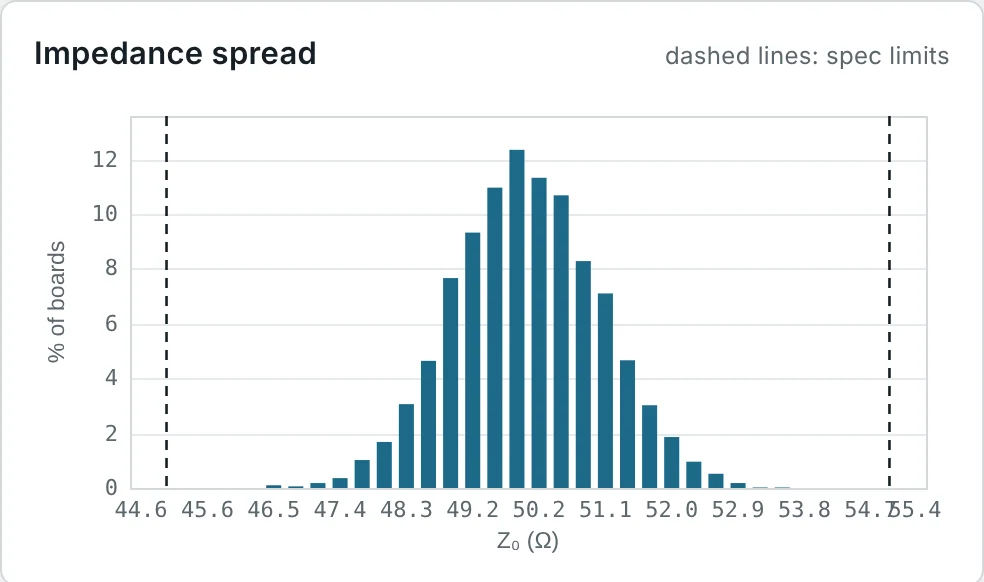
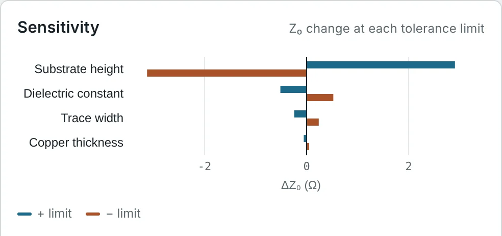
The last point is critical for PCB design. Fig 3 shows a Monte Carlo analysis from the microstrip calculator for the 50 Ω FR-4 line, with typical fabrication tolerances: trace width ±25 µm, substrate height ±10%, εr ±0.10 and copper thickness ±5 µm. The impedance spread has a standard deviation of 1.0 Ω (±3σ = ±6%), and the sensitivity chart shows that the substrate height dominates — a 10% thickness change moves Z₀ by about 3 Ω, six times more than the dielectric-constant tolerance. This is why fabricators sell "controlled impedance" boards with a ±10% or ±5% specification and adjust the etched width to compensate for the laminate actually used.

Histogram of microstrip characteristic impedance over 5000 simulated FR-4 boards, centred at 50 ohms with a standard deviation of about 1 ohm — Fig 3a — Z₀ over 5,000 simulated boards: mean 49.98 Ω, σ = 1.01 Ω, 1st–99th percentile 47.7–52.3 Ω. Try it in the Microstrip & Stripline Impedance Calculator →

Tornado chart of impedance change at each tolerance limit: substrate height about plus or minus 3 ohms, dielectric constant about 0.5 ohm, trace width about 0.25 ohm, copper thickness negligible — Fig 3b — Sensitivity: substrate height dominates, followed by εr, trace width and copper thickness. Try it in the Microstrip & Stripline Impedance Calculator →

Characteristic Impedance vs Load Impedance

Z₀ belongs to the line; the load impedance Z_L belongs to whatever is connected at the end. Their relationship decides what happens to the wave at the load, through the reflection coefficient:

Reflection at the load

Γ = \frac{Z_{L} - Z_{0}}{Z_{L} + Z_{0}}

RL = - 20 \log_{10} | Γ |

ML = - 10 \log_{10} (1 - | Γ |^{2})

Γ = 0 only when Z_L = Z₀. A purely resistive load R_L gives VSWR = R_L/Z₀ or Z₀/R_L, whichever is larger.

Three consequences are worth separating clearly:

The impedance seen at the input depends on Z₀, Z_L and the electrical length — unless Z_L = Z₀, in which case it is Z₀ at every length and every frequency. That is the practical meaning of "matched": a matched line is invisible.
A mismatch costs power (mismatch loss ML) and, on a transmitter, can damage the output stage through high VSWR.
Z₀ itself can be any value — a 75 Ω line is just as good as a 50 Ω line if the source and load are 75 Ω. Problems arise only at the boundaries between different impedances, including connectors and changes of line width (Part 13).

Mismatches and their correction are the subject of the Smith chart series; Part 7 derives the input impedance of a terminated line.

Measuring Characteristic Impedance

Because Z₀ is not a resistance, it is measured indirectly. Three methods are common:

Derivation — the open/short method: Z₀ = √(Z_ocZ_sc)

Measure the input impedance of a length ℓ of lossless line twice, once with the far end short-circuited and once open. From the input-impedance formula of Part 7 with Z_L = 0 and Z_L = ∞:

Z_{s c} = j Z_{0} \tan β ℓ Z_{o c} = - j Z_{0} \cot β ℓ

Their product removes the length dependence, and their ratio gives the electrical length:

Open/short method

Z_{0} = \sqrt{Z_{o c} Z_{s c}} \tan β ℓ = \sqrt{- \frac{Z_{s c}}{Z_{o c}}}

The result holds for lossy lines too, with tan βℓ replaced by tanh γℓ. Avoid lengths near a multiple of λ/4, where one of the two readings is very large and inaccurate.

Time-domain reflectometry (TDR). Launch a fast step from a known Z_s (usually 50 Ω) and measure the reflected step. Each section of line shows up at a delay set by its position, with Γ = (Z₀ − Z_s)/(Z₀ + Z_s). TDR is the standard way PCB fabricators verify controlled-impedance coupons.
Capacitance and delay. Z₀ = τ/C for a length of line, with C measured at low frequency and τ from a pulse or the frequency of the first quarter-wave resonance.
Vector network analyser. Measure S-parameters of a line section and extract Z₀ and γ from them — the most accurate method at microwave frequencies.

Practical Characteristic Impedance Calculations

The worked examples below use c = 2.998 × 10⁸ m/s and η₀ = 376.7 Ω.

Identifying an Unknown Cable from C and Delay

Problem: A 1.00 m length of unmarked coax measures 67 pF between its conductors, and a pulse takes 5.05 ns to travel through it. Find Z₀, L′ and the velocity factor.

Z₀ = τ/C and L′ = Z₀²C′

Z_{0} = \frac{τ}{C} = \frac{5.05 \times 10^{- 9}}{67 \times 10^{- 12}} = 75.4 Ω

L^{'} = Z_{0}^{2} C^{'} = {75.4}^{2} \times 67 \times 10^{- 12} = 381 nH/m

Velocity factor

v_{p} = \frac{1.00 m}{5.05 ns} = 1.98 \times 10^{8} m/s

VF = \frac{1.98}{2.998} = 0.66

Answer: a 75 Ω cable with solid-PE dielectric (VF 0.66, εr ≈ 2.3)

RG-59 and RG-6 with solid PE match this description. The method needs no RF equipment — a capacitance meter and an oscilloscope suffice.

Lossy Z₀ of RG-58 at Low Frequency

Problem: RG-58 has L′ = 258.5 nH/m, C′ = 96.8 pF/m and a DC loop resistance of 0.045 Ω/m. Find Z₀ at 1 kHz and at 100 kHz (R′ = 0.061 Ω/m including skin effect).

1 kHz: ωL′ = 0.0016 Ω/m ≪ R′

Z_{0} = \sqrt{\frac{0.0456 + j 0.0016}{j 6.08 \times 10^{- 7}}} = 274 ∠ - 44^{\circ} Ω

100 kHz: ωL′ = 0.162 Ω/m, about 2.7 R′

Z_{0} = \sqrt{\frac{0.061 + j 0.162}{j 6.08 \times 10^{- 5}}} = 53.4 ∠ - {10.3}^{\circ} Ω

Answer: 274∠−44° Ω at 1 kHz; 53.4∠−10° Ω at 100 kHz; 51.7 Ω above about 1 MHz

"50 Ω" cable is 50 Ω only at RF. An audio engineer driving a long coax run, or a designer of a DC-to-GHz instrument, must allow for the complex low-frequency Z₀ shown in Fig 2.

The Imaginary Part of Z₀ on a Low-Loss Line

Problem: The coax of Part 3, Example 1 has R′ = 0.8 Ω/m, L′ = 250 nH/m, G′ = 0.1 mS/m and C′ = 100 pF/m. Use the low-loss formula to find Z₀ at 1 GHz.

Correction term

\frac{1}{2 ω} (\frac{R^{'}}{L^{'}} - \frac{G^{'}}{C^{'}}) = \frac{1}{2 \times 6.283 \times 10^{9}} (3.2 \times 10^{6} - 1.0 \times 10^{6}) = 1.75 \times 10^{- 4}

Z₀

Z_{0} \approx 50 (1 - j 1.75 \times 10^{- 4}) = 50.000 - j 0.0088 Ω = 50.000 ∠ - {0.010}^{\circ} Ω

Answer: Z₀ = 50.000 − j0.009 Ω — identical to the exact result

Because R′/L′ > G′/C′ (conductor loss dominates), the small imaginary part is negative (capacitive). Adding a little loading inductance, or a little dielectric loss, would move the line towards Heaviside's distortionless condition and make it zero.

Measuring Z₀ with Open and Short Terminations

Problem: A VNA measures a length of cable at 100 MHz as Z_sc = j35.1 Ω with the far end shorted and Z_oc = −j71.2 Ω with it open. Find Z₀ and the electrical length.

Characteristic impedance

Z_{0} = \sqrt{(- j 71.2) (j 35.1)} = \sqrt{2499} = 50.0 Ω

Electrical length

\tan β ℓ = \sqrt{\frac{35.1}{71.2}} = 0.702 \Rightarrow β ℓ = {35.1}^{\circ} (or {35.1}^{\circ} + n \times 180^{\circ})

Answer: Z₀ = 50.0 Ω; electrical length 35.1° (plus any multiple of 180°)

The ambiguity of n × 180° is resolved by repeating the measurement at a slightly different frequency or from the approximate physical length. The method works with any impedance analyser and needs no 50 Ω reference.

Designing a 75 Ω Foam Coax

Problem: A 75 Ω satellite-TV cable uses gas-injected foam PE (εr = 1.5) and a 1.0 mm diameter centre conductor. What diameter must the foam dielectric be?

Invert Z₀ = (60/√εr) ln(b/a)

\frac{b}{a} = \exp (\frac{75 \sqrt{1.5}}{60}) = e^{1.531} = 4.62

2 b = 4.62 \times 1.0 = 4.62 mm

Answer: a foam diameter of about 4.6 mm

RG-6 satellite cable has a 1.0 mm centre conductor and a 4.6–4.7 mm foam dielectric — exactly this. With solid PE (εr = 2.25) the dielectric would have to be 6.5 mm across for the same 75 Ω, which is why foam both lowers the loss and shrinks the cable.

Impedance Tolerance of a 50 Ω FR-4 Trace

Problem: For the 3.07 mm, 50 Ω microstrip on 1.6 mm FR-4 (35 µm copper), estimate Z₀ at the limits of (a) ±50 µm etch tolerance, (b) εr = 4.1–4.5 and (c) ±10% substrate height. Which matters most?

Hammerstad–Jensen at each limit

(a) w \pm 50 μ m : 49.5 – 50.5 Ω

(b) ε_{r} 4.5 – 4.1 : 49.0 – 51.1 Ω

(c) h 1.44 – 1.76 mm : 46.9 – 52.9 Ω

Answer: height ±10% gives ±3 Ω, εr ±5% gives ±1 Ω, width ±50 µm only ±0.5 Ω

On a thick board with wide traces the dielectric height and εr dominate; on thin boards with narrow traces the etch tolerance becomes the largest term. Matching Fig 3b, the first item on a controlled-impedance specification should be the dielectric thickness between the trace and its reference plane.

Spacing of a 300 Ω Twin-Lead

Problem: What centre spacing D gives 300 Ω for two 1.0 mm diameter wires in air? How does a polyethylene web that raises εeff to 1.3 change the impedance?

Air line

\cosh^{- 1} \frac{D}{2 a} = \frac{300 π}{376.7} = 2.502 \Rightarrow \frac{D}{2 a} = 6.14, D = 6.14 mm

With the web

Z_{0} = \frac{300}{\sqrt{1.3}} = 263 Ω

Answer: D ≈ 6.1 mm in air; the web lowers Z₀ to about 263 Ω unless D is increased

Commercial 300 Ω ribbon uses a wider spacing (about 8–10 mm for thinner wire) to compensate for the web. Moisture on the web raises εeff further — the reason twin-lead's impedance drifts in rain.

Connecting a 75 Ω Device to a 50 Ω System

Problem: A 75 Ω video receiver is connected to a 50 Ω generator through 50 Ω cable. Find Γ, the return loss, the VSWR and the mismatch loss.

Reflection

Γ = \frac{75 - 50}{75 + 50} = 0.20 RL = - 20 \log 0.2 = 14.0 dB VSWR = 1.5

Mismatch loss

ML = - 10 \log_{10} (1 - 0.04) = 0.18 dB

Answer: Γ = 0.2, RL = 14 dB, VSWR = 1.5, ML = 0.18 dB

Only 4% of the power is reflected, so for many purposes a 50/75 Ω mismatch is tolerable. For precision measurements a minimum-loss matching pad (5.7 dB loss) is used instead.

Why a Matched Line Is Invisible

Problem: A 10 m, 50 Ω line is terminated (a) in 50 Ω and (b) in 75 Ω. Between what limits can the input impedance lie as the frequency (and so the electrical length) varies?

(a) Matched: Γ = 0

Z_{i n} = 50 Ω at every frequency

(b) VSWR S = 1.5: Z_in swings between real extremes Z₀/S and Z₀S

\frac{Z_{0}}{S} = 33.3 Ω \leq | Z_{i n} | at the real points \leq Z_{0} S = 75 Ω

Answer: (a) always 50 Ω; (b) between 33.3 Ω and 75 Ω (and complex values in between), repeating every λ/2

With a matched load the line has no effect on the impedance, so any length can be used. With a mismatch the source sees an impedance that depends on cable length and frequency — the reason that cable length "matters" only in mismatched systems.

Measuring a PCB Coupon by TDR

Problem: A TDR with a 50 Ω source launches a 250 mV step into a PCB test coupon. The reflection from the coupon trace is a +27 mV step. What is the trace impedance? Is it within a 50 Ω ± 10% specification?

Reflection coefficient and impedance

Γ = \frac{27}{250} = 0.108

Z_{0} = Z_{s} \frac{1 + Γ}{1 - Γ} = 50 \times \frac{1.108}{0.892} = 62.1 Ω

Answer: Z₀ ≈ 62 Ω — outside the 45–55 Ω specification

The trace is about 24% high, typically caused by a thinner-than-specified trace or a thicker dielectric. Fabricators make exactly this measurement on a coupon at the edge of each panel and adjust the etch compensation until the coupons pass.

Summary

Z₀ is the voltage-to-current ratio of a single travelling wave, and the input impedance of an infinite line or of any line terminated in Z₀.
From the infinite ladder: Z₀ = √((R′ + jωL′)/(G′ + jωC′)). Lossless: Z₀ = √(L′/C′), real and frequency-independent.
Low-loss: Z₀ ≈ √(L′/C′)[1 − (j/2ω)(R′/L′ − G′/C′)]. At low frequency Z₀ → √(R′/jωC′), with an angle near −45°.
Z₀ = v_pL′ = 1/(v_pC′) = τ/C; L′ = Z₀√εeff/c and C′ = √εeff/(cZ₀).
50 Ω is the compromise between the 30 Ω power optimum and the 77 Ω loss optimum of air coax; 75 Ω is used where loss matters most.
Z₀ is set by geometry and εr; on PCBs the dielectric thickness usually dominates its tolerance.
Measure Z₀ with Z₀ = √(Z_ocZ_sc), with TDR, or from capacitance and delay.

Z₀ describes the relation between voltage and current in a wave; the propagation constant describes how the wave itself changes as it travels. Part 5: Propagation Constant, Phase Velocity and Group Velocity examines γ in detail — attenuation, phase constant, phase and group velocity, and dispersion.

📘 Go deeper: Z₀ on the Smith chart

Every point on the Smith chart is an impedance normalised to Z₀ — the chart only works once Z₀ is known. Open Smith Chart & Impedance Matching series →

Put It Into Practice

Use the NEXT ANTENNAS calculators to apply the ideas from this article to real lines and circuits.

Transmission Lines Microstrip & Stripline Impedance Calculator Field-solver backed design of microstrip, embedded microstrip, stripline, GCPW and differential pairs: width, εeff, Z₀, loss, dispersion and tolerance. Open calculator → Impedance Matching Smith Chart Visualiser Plot impedances, move along lines and stubs, load Touchstone files and design matching networks. Open calculator → Link & Power VSWR & Return Loss Calculator Convert between VSWR, return loss, reflection coefficient and mismatch loss. Open calculator → All Tools All RF Calculators Browse every NEXT ANTENNAS calculator for RF, microwave and antenna design. Open calculator →

Characteristic Impedance of Transmission Lines