Introduction to Microstrip Transmission Lines
Open almost any wireless product — a phone, a Wi-Fi router, a GPS receiver, a radar module — and the RF signals between the chips, filters and antenna travel on microstrip: a copper trace on the top layer of a printed circuit board with a solid ground plane underneath. Microstrip is cheap (it is made by the same photo-etching process as any PCB), it is open on top so that components can be soldered directly onto it, and its impedance is set by a single dimension, the trace width. Filters, couplers, power dividers, matching networks and patch antennas are all built from it.
The price of that convenience is that microstrip is the most awkward of the common lines to analyse. Its field lives partly in the substrate and partly in the air above, so it does not carry a pure TEM wave, its phase velocity changes slightly with frequency, and there is no exact closed-form expression for its characteristic impedance. This article builds the theory step by step, using the ideas from the earlier parts of this series: the RLGC model of Part 3, the characteristic impedance of Part 4, the propagation constant and phase velocity of Part 5, guided wavelength from Part 6, and the loss mechanisms of Part 8.
Throughout the article the formulas are checked against the NEXT ANTENNAS Microstrip & Stripline Impedance Calculator, which solves the 2D field problem with the finite element method (FEM) and also evaluates the standard closed-form models. Two reference boards are used: 1.6 mm FR-4 (εr = 4.3, tan δ = 0.02) and 0.813 mm Rogers RO4003C (design εr = 3.55, tan δ = 0.0027), both with 35 µm (1 oz) copper.
Microstrip Structure and Geometry
A microstrip has three parts: a signal strip of width w and thickness t, a dielectric substrate of height h, relative permittivity εr and loss tangent tan δ, and a ground plane covering the whole underside (Fig 1). The return current flows in the ground plane directly beneath the strip, so the strip and the ground together form the two conductors that every TEM-like line needs.
Five numbers describe a microstrip electrically:
- w/h — the width-to-height ratio. This, more than anything else, sets the characteristic impedance: wide strips (w/h > 1) give low impedance, narrow strips give high impedance.
- εr — the substrate permittivity. Higher εr concentrates the field in the substrate, lowers Z₀ for a given w/h, and shortens the guided wavelength.
- t/h — the normalised copper thickness. It makes the strip look slightly wider than it is, a small correction for 17–35 µm copper on boards thicker than about 0.25 mm.
- tan δ and the copper conductivity σ and roughness — these set the attenuation, not the impedance.
- f·h — the product of frequency and substrate height. It sets how far the line departs from its low-frequency behaviour (dispersion) and where it stops working as a single-mode line.
The substrate is chosen first, usually for loss, cost and permittivity tolerance; the width is then designed for the impedance. Typical RF substrates are listed below.
| Substrate | εr (design) | tan δ | Common heights | Typical use |
|---|---|---|---|---|
| FR-4 (glass–epoxy) | 4.2–4.6 | 0.015–0.02 | 0.2–1.6 mm | Low-cost boards below about 3 GHz, digital |
| Rogers RO4003C | 3.55 | 0.0027 (10 GHz) | 0.203–1.524 mm | Mainstream RF and microwave, FR-4-compatible processing |
| Rogers RO4350B | 3.66 | 0.0037 (10 GHz) | 0.101–1.524 mm | Power amplifiers, base stations |
| RT/duroid 5880 (PTFE) | 2.20 | 0.0009 (10 GHz) | 0.127–3.175 mm | Low-loss microwave and mm-wave, antennas |
| RO3010 (ceramic-filled PTFE) | 10.2 | 0.0022 (10 GHz) | 0.13–1.28 mm | Miniaturised filters and circuits |
| Alumina (99.6%) | 9.8–9.9 | ≈0.0001 | 0.254–0.635 mm | Thin-film hybrid microwave circuits |
Laminate datasheets often list two permittivities. The process value (3.38 for RO4003C) is measured by a clamped-stripline test; the design value (3.55) is extracted from real microstrip circuits and already includes effects such as the anisotropy of the glass weave. Use the design value for microstrip impedance calculations.
Electric and Magnetic Field Distribution
The strip and ground plane carry equal and opposite currents and charges. The electric field starts on the charge of the strip and ends on the opposite charge in the ground plane. Directly under the strip, where the strip and ground face each other, the field is almost uniform and vertical — this is the "parallel-plate" part of the line. Beyond the strip edges the field lines bow outwards (fringing), and some of them leave the substrate, arc through the air above, and come back down to the ground plane. The magnetic field circles the strip, as it does around any current-carrying conductor, and is squeezed into the region between strip and ground.
Fig 2 shows the field from the calculator's FEM solution of the 50 Ω FR-4 line. The left panel shows equipotential bands of the quasi-static potential — the potential is highest on the strip and falls to zero at the ground. The right panel shows the magnitude of the electric field on a log scale: it is strongest under the strip and at the strip's two edges, where the charge (and the current) crowds onto the corners.
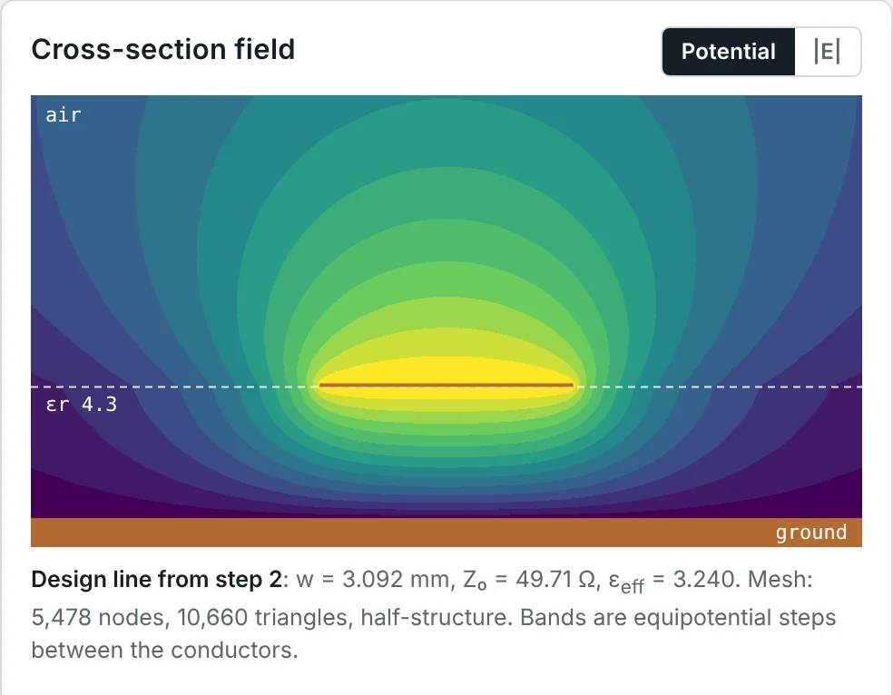
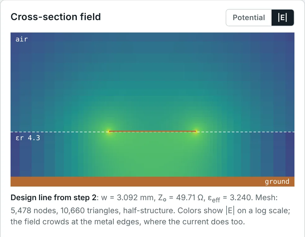
Two consequences follow directly from this picture:
- The wave sees a mixture of air and dielectric. Some of the electric energy is stored in the substrate and some in the air, so the wave travels faster than it would in a fully filled line but slower than in air. This mixture is described by the effective dielectric constant εeff.
- The current is not uniform across the strip. It peaks near the edges and is spread out in the ground plane under the strip. Edge crowding raises the conductor loss above the value you would calculate from a uniform current.
The Quasi-TEM Mode of Propagation
A coaxial cable or a stripline is filled with a single, uniform dielectric, and it carries a true TEM wave: E and H are entirely transverse and the wave travels at v = c/√εr. Microstrip cannot do this. A TEM wave would have to travel at c in the air and at c/√εr in the substrate at the same time, but the fields on both sides of the interface are tied together by the boundary conditions, so they must share one propagation constant β. The only way to satisfy Maxwell's equations at the interface is to add small longitudinal (z-directed) field components.
Let the interface be the plane y = h, with the wave travelling along z as e−jβz. Take the x-component of Ampère's law, ∇ × H = jωεE, on each side of the interface:
At the interface the tangential electric field is continuous, Exd = Exa, and because both media have permeability μ₀ the normal magnetic field Hy is continuous too (see the boundary-conditions article). Multiply the air equation by εr and subtract the substrate equation; Ex cancels:
The longitudinal fields are proportional to (εr − 1) and to β, and they are significant only when the substrate is electrically thick. For h ≪ λ the transverse fields dominate and the mode behaves almost exactly like a TEM wave — hence the name quasi-TEM.
In practice this has a very useful consequence. At frequencies where h is a small fraction of a wavelength, the transverse field pattern is almost identical to the static field you would get by putting a DC voltage between the strip and the ground. Everything about the line — its capacitance, its inductance, Z₀ and εeff — can therefore be computed from a 2D electrostatic problem. This is the quasi-static approximation, and it is exactly what the calculator's FEM solver does. The departure from it at higher frequencies is the dispersion covered later in this article.
Effective Dielectric Constant
The quasi-static approximation turns microstrip analysis into two capacitance calculations. Let C be the capacitance per unit length of the actual line and Ca the capacitance per unit length of the same line with the substrate replaced by air. Because the substrate is non-magnetic, the inductance per unit length L is the same in both cases — the magnetic field does not "see" the dielectric.
The air-filled version of the line is a true TEM line in a homogeneous medium, so its wave travels at c (Part 5):
The real line has the same L but capacitance C, so its phase velocity and impedance are
Defining the effective dielectric constant by vp = c/√εeff gives the two key results:
The calculator's FEM solver uses exactly these relations: it solves Laplace's equation twice, once with the substrate and once in air, and reports εeff = C/Ca and Z₀ = 1/(c√(C·Ca)).
The filling factor and the limits of εeff
It is helpful to write εeff in terms of a filling factor q — roughly, the fraction of the electric field energy that is stored in the substrate:
Fig 3 plots q against w/h for four common permittivities. For practical 50 Ω lines (w/h between 1 and 3), q is between about 0.64 and 0.73 — so roughly two-thirds to three-quarters of the field is in the substrate. Note that q depends only weakly on εr: the geometry, not the material, decides how the field divides.
The most widely used closed-form expression for εeff — accurate to about 1% and simple enough for hand calculation — is the one popularised by Hammerstad and given in Pozar's Microwave Engineering:
Characteristic Impedance of Microstrip Lines
The characteristic impedance is the ratio of voltage to current in a single travelling wave (Part 4). For microstrip there is no exact formula, but two limiting cases can be derived by hand, and they explain the shape of every design curve.
When w ≫ h the field under the strip is uniform, like a parallel-plate capacitor, and fringing can be ignored. Per unit length the capacitance and inductance are those of a parallel-plate line of width w and spacing h:
Fringing adds capacitance at each edge, so a real strip behaves as if it were wider. Wheeler showed that the effective width is w + h·[1.393 + 0.667 ln(w/h + 1.444)], which leads to the wide-strip formula below.
When w ≪ h the strip looks like a thin wire at height h over the ground plane. By image theory, a wire of radius a at height h over ground is half of a two-wire line with spacing 2h, so its impedance is half of (η₀/π)·ln(2h/a). A flat strip of width w has the same capacitance as a round wire of radius a ≈ w/4, which gives
Joining these two limits with fitted correction terms gives the standard analysis formulas. Use the first for narrow strips and the second for wide ones; they agree at w/h = 1:
For software, the more accurate Hammerstad–Jensen (1980) model is the industry standard; it is accurate to about 0.2% for zero-thickness strips over 0.01 ≤ w/h ≤ 100 and εr ≤ 128. With u = w/h:
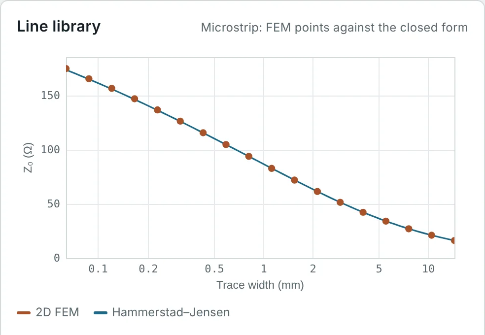
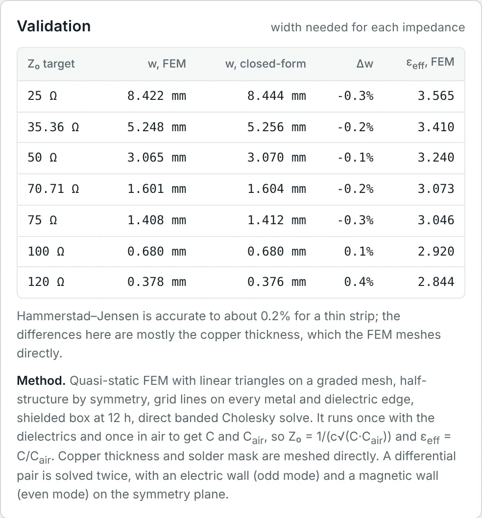
How good are these formulas? Fig 5 compares the Hammerstad–Jensen curve with the FEM solution for the FR-4 board across the whole practical range of widths, and tabulates the width each method needs for seven standard impedances. The two agree to within 0.4%; the small remaining differences come mainly from the 35 µm copper thickness, which the FEM meshes directly.
Microstrip Width and Substrate Thickness
Look again at the formulas above: Z₀ and εeff depend on w and h only through their ratio w/h (and on t only through t/h). This is not a coincidence of the curve fits. In the quasi-static approximation Z₀ is fixed by the capacitances C and Ca, and capacitance per unit length is dimensionless apart from the factor ε₀ — scaling every dimension of the cross-section by the same factor leaves it unchanged. So:
In practice the substrate height is chosen from a short list of standard laminate thicknesses, and the trace width follows. Very thin substrates (below about 0.2 mm) give 50 Ω traces narrower than 0.4 mm, which raises the conductor loss and makes the impedance more sensitive to etching tolerance; very thick ones give wide traces that do not fit between the pads of small components and push the upper frequency limit down.
Effect of the Dielectric Constant on Impedance
Raising εr increases the capacitance C while leaving the inductance unchanged, so Z₀ = √(L/C) falls. For a fixed impedance the trace must therefore be narrower on a high-εr substrate, as Fig 4 showed. At the same time the guided wavelength shrinks as 1/√εeff, so every quarter-wave transformer, stub and resonator becomes shorter.
| Substrate εr (h = 0.508 mm) | 50 Ω width | w/h | εeff | λg at 5 GHz |
|---|---|---|---|---|
| 2.2 (PTFE) | 1.566 mm | 3.08 | 1.881 | 43.7 mm |
| 3.0 | 1.277 mm | 2.51 | 2.425 | 38.5 mm |
| 3.55 (RO4003C) | 1.137 mm | 2.24 | 2.787 | 35.9 mm |
| 6.15 (RO3006) | 0.748 mm | 1.47 | 4.413 | 28.5 mm |
| 10.2 (RO3010) | 0.474 mm | 0.93 | 6.793 | 23.0 mm |
Two further points matter in practice. First, high-εr substrates hold more of the field inside the board, so the line radiates less and couples less to neighbouring traces — an advantage for dense circuits. Second, the tolerance on εr translates directly into impedance error: since Z₀ ∝ 1/√εeff and εeff ≈ 1 + q(εr − 1), a ±5% spread in εr on FR-4 (4.1–4.5) gives roughly ±2% in Z₀, and a larger error in the electrical length of resonant structures. This is one of the main reasons microwave designs move from FR-4 to controlled-εr laminates.
Effect of Substrate Thickness on Impedance
For a fixed trace width, increasing the substrate height moves the strip further from its ground, reducing C and increasing L, so the impedance rises. The table below shows a 0.5 mm wide trace on RO4003C laminates of the standard thicknesses, together with the width each one needs for 50 Ω.
| RO4003C height h | Z₀ of a 0.5 mm trace | 50 Ω width | w/h for 50 Ω |
|---|---|---|---|
| 0.203 mm (8 mil) | 47.0 Ω | 0.454 mm | 2.24 |
| 0.305 mm (12 mil) | 60.2 Ω | 0.682 mm | 2.24 |
| 0.508 mm (20 mil) | 78.6 Ω | 1.137 mm | 2.24 |
| 0.813 mm (32 mil) | 96.5 Ω | 1.819 mm | 2.24 |
| 1.524 mm (60 mil) | 121.1 Ω | 3.410 mm | 2.24 |
This table is also the reason that a microstrip's impedance depends on the actual pressed thickness of the dielectric between the trace and its reference plane — in a multilayer board, that is the prepreg or core between layer 1 and layer 2, not the total board thickness. A common layout mistake is to calculate the width for a 1.6 mm board when the reference plane is on layer 2, only 0.2 mm below: the result is a 50 Ω calculation that produces a roughly 110 Ω trace.
Microstrip Design Equations
The analysis formulas give Z₀ from w/h. In design we need the reverse: the w/h that gives a target Z₀. Wheeler's synthesis equations, in the form given by Pozar, invert the analysis formulas to about 1%:
Correcting for copper thickness
A strip of finite thickness has extra capacitance from its side walls, so it behaves as if it were slightly wider. A simple correction, adequate for w/h ≥ 1/(2π), increases the effective width by
A practical design procedure
- Choose the substrate for loss, cost and εr tolerance, and find the dielectric height between the trace and its reference plane (from the stack-up, not the board thickness).
- Synthesise w/h with the Wheeler equations (or the calculator), using the design εr at the operating frequency.
- Correct for copper thickness and, if there is one, for solder mask over the trace (which lowers Z₀ by 1–3 Ω on a 50 Ω line).
- Check εeff and the guided wavelength at the operating frequency, including dispersion, before drawing any resonant length.
- Check the upper frequency limit and the loss for the highest frequency of interest.
- Check manufacturing tolerance: etched widths are typically ±25–50 µm and laminate heights ±5–10%; the calculator's tolerance pane gives the resulting spread in Z₀.
Microstrip Dispersion
The quasi-static values of εeff and Z₀ hold only at low frequency. As the frequency rises, the longitudinal field components found in the quasi-TEM derivation grow, and the field pulls itself down into the substrate — the region where the wave would naturally travel more slowly. The filling factor increases, and εeff rises from its quasi-static value towards εr. In the limit of very high frequency all the field is in the substrate and εeff → εr.
Because the phase velocity c/√εeff(f) now depends on frequency, microstrip is dispersive: different frequency components of a signal travel at slightly different speeds (Part 5 covers phase and group velocity). For narrowband circuits the main practical effect is that resonant lengths designed with the quasi-static εeff come out slightly too long.
A simple model that captures the physics and is easy to use by hand is Getsinger's:
Modern CAD tools and the calculator use the more accurate Kirschning–Jansen model (accurate to about 0.6% for substrates up to about 0.13 λ₀ thick). Its structure is the same — εeff(f) = εr − (εr − εeff(0))/(1 + P(f)) — with P a fitted function of w/h, εr and the normalised frequency f·h. That last variable confirms the scaling rule: dispersion depends on frequency and substrate height only through their product.
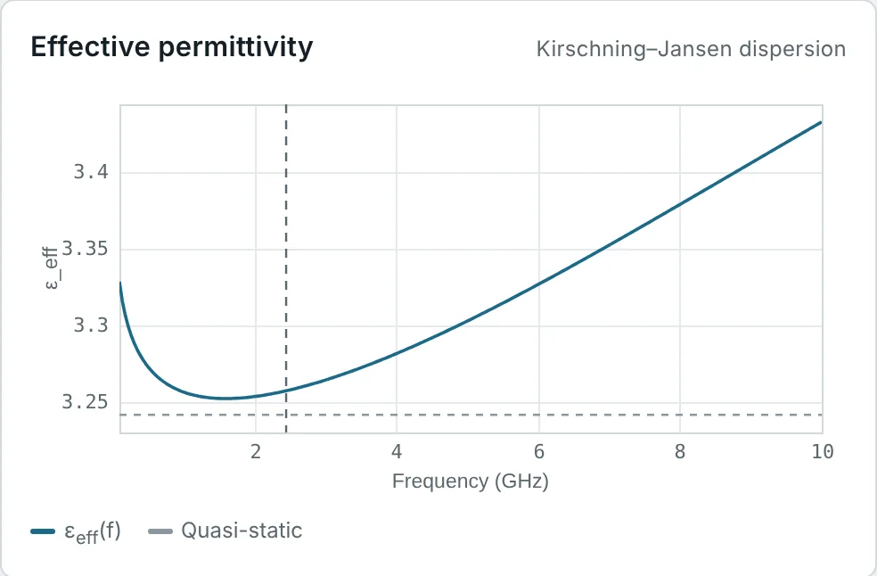
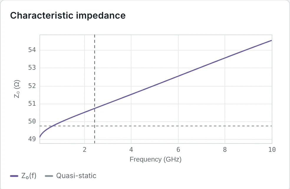
Real laminates add a second, material dispersion: the permittivity of the substrate itself falls slowly with frequency. FR-4 is the extreme case — its datasheet Dk of 4.30 at 1 GHz has dropped to about 4.25 at 2.45 GHz and falls further at 10 GHz. The calculator models this with a wideband Debye (Djordjevic–Sarkar) material, and Fig 7 shows the result for the 50 Ω FR-4 line: at low frequency εeff first falls as the material Dk drops, then rises as geometric dispersion takes over. The impedance rises slowly with frequency at the same time.
Higher-Order Modes, Surface Waves and the Upper Frequency Limit
Dispersion is gradual, but three effects set a hard upper frequency for a microstrip line:
- Transverse resonance. The strip and ground form a parallel-plate resonator across the width of the line. When the effective width (about w + 0.4h on each side) reaches half a wavelength in the substrate, the first higher-order microstrip mode propagates, and the line no longer carries a single, well-defined wave.
- Surface waves. A grounded dielectric slab can guide surface waves even with no strip on it. The lowest (TM₀) surface wave has no cutoff; the quasi-TEM mode couples strongly to it, and leaks power into it, once their phase velocities approach each other. The first TE surface wave starts at fTE1.
- Radiation. Discontinuities such as bends, open ends and steps radiate a fraction of the power that grows as (h/λ)², which is why thick substrates make good patch antennas but poor high-frequency circuits.
For most practical 50 Ω lines the transverse resonance is the lowest limit. All three are inversely proportional to h, which is why mm-wave circuits use substrates only 0.1–0.25 mm thick.
Conductor and Dielectric Losses
A microstrip loses power in three ways: resistive loss in the strip and ground (conductor loss αc), polarisation loss in the substrate (dielectric loss αd), and radiation. The total attenuation is α = αc + αd + αr in nepers per metre; multiply by 8.686 to get dB/m. Part 8 derives these mechanisms for a general line; here we apply them to microstrip.
Treat the substrate permittivity as complex, εr(1 − j tan δ), and apply the filling-factor relation to the complex value. Only the substrate part carries loss, so the effective permittivity becomes
For a low-loss medium the attenuation is αd = (β/2) tan δeff with β = k₀√εeff. Substituting q = (εeff − 1)/(εr − 1):
At RF the current flows in a skin depth δs = 1/√(πfμ₀σ), and a conductor of width w presents a surface resistance Rs = √(πfμ₀/σ) per square. Approximating the microstrip by a parallel-plate line of width w, the strip and the ground each contribute Rs/w, so R = 2Rs/w per metre. For a low-loss line αc = R/(2Z₀) (Part 5), which gives
The parallel-plate picture ignores two effects that roughly cancel for typical 50 Ω lines: current crowding at the strip edges (which increases the loss) and the spreading of the ground current over a width larger than w (which reduces it). Full models such as Pucel's or Wheeler's incremental-inductance rule, used by the calculator, account for both.
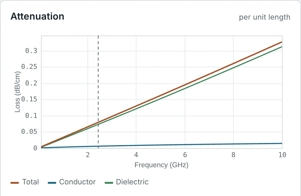
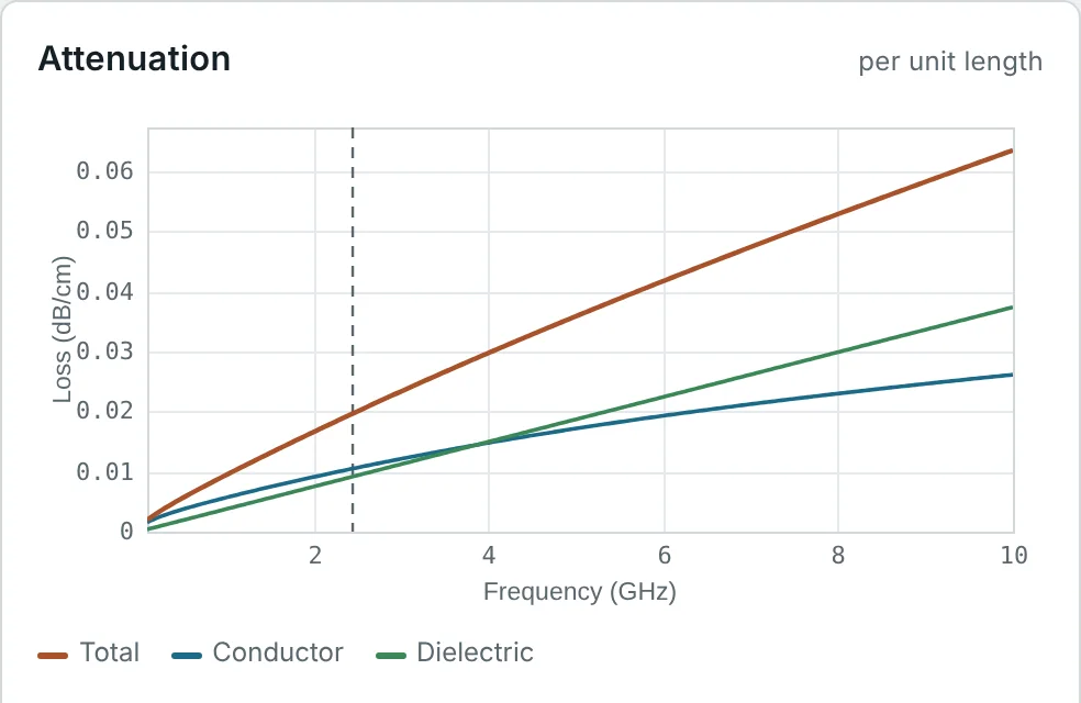
Fig 8 compares the loss breakdown of the two reference lines. On FR-4 the dielectric dominates — at 2.45 GHz it is 92% of the total, 0.073 of 0.080 dB/cm — because tan δ = 0.02 is very high. On RO4003C the dielectric loss is eight times smaller, and the conductor loss becomes comparable to it; the total is 0.020 dB/cm at 2.45 GHz, a quarter of FR-4's. This is the strongest single reason for using a microwave laminate.
To reduce microstrip loss: use a low-tan δ substrate (the biggest effect at microwave frequencies), use a thicker substrate so the 50 Ω trace is wider (lower αc), specify smooth (rolled or reverse-treated) copper above a few GHz, keep traces short, and avoid unnecessary discontinuities that radiate.
Practical Microstrip Impedance Calculations
Most RF boards need only a handful of impedances: 50 Ω for interconnects, the quarter-wave transformer values 35.36 Ω and 70.71 Ω (to match 25 Ω and 100 Ω loads to 50 Ω), and occasionally 25, 75 and 100 Ω for stubs, couplers and filters. The calculator's design pane tabulates them for any board at the design frequency, including dispersion, together with the physical length of a quarter-wave section.
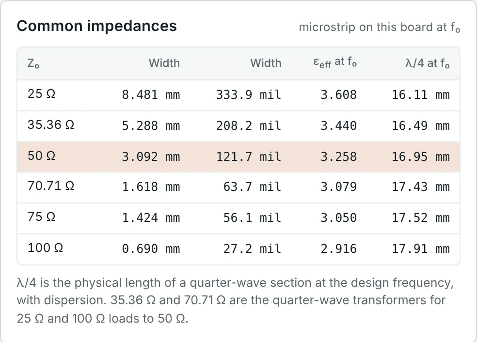
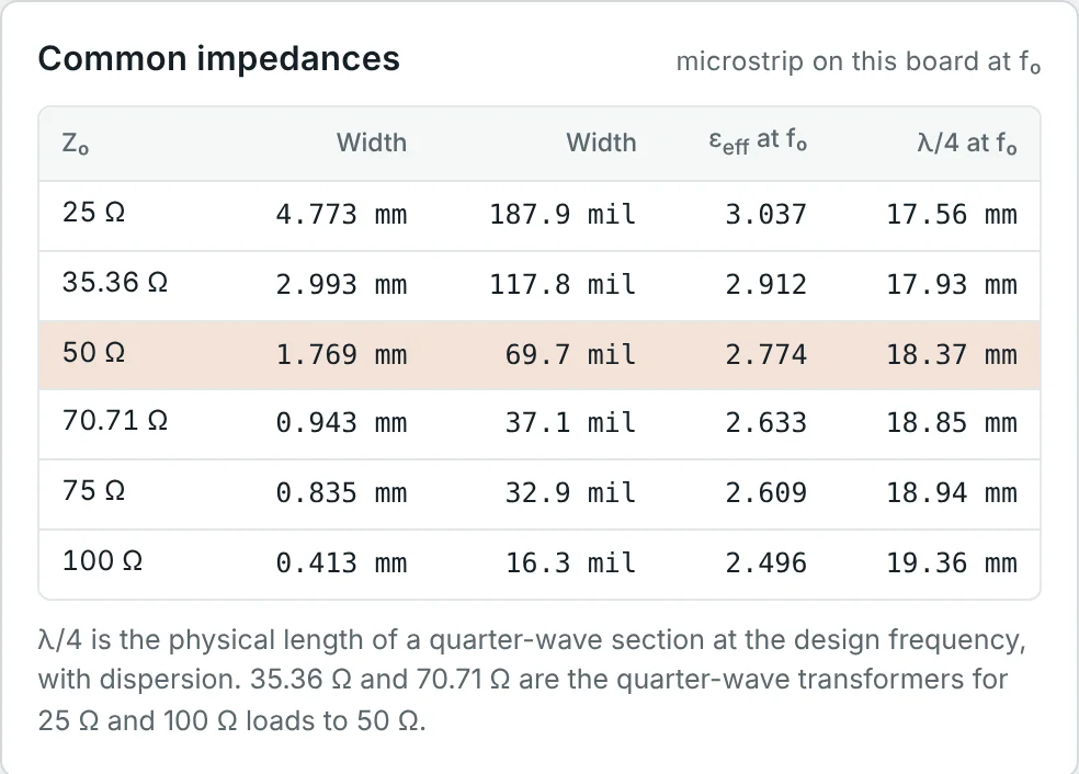
Notice how the quarter-wave length increases as the impedance rises: narrower, higher-impedance lines have a lower filling factor, a lower εeff, and therefore a longer guided wavelength. A 100 Ω quarter-wave section on FR-4 is 17.91 mm long; a 25 Ω section is 16.11 mm — an 11% difference that a design using a single "board εeff" would miss.
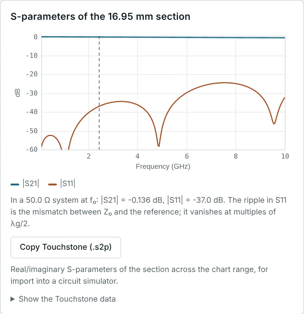
Finally, the calculator converts the line into a two-port. Fig 10 shows the S-parameters of the 16.95 mm quarter-wave section of 50 Ω FR-4 line in a 50 Ω system. The insertion loss at 2.45 GHz is 0.136 dB; the small S₁₁ (−37 dB) comes from the difference between the line's dispersive Z₀ and the 50 Ω reference, and it vanishes wherever the line is a multiple of λg/2 long (near 4.9 and 9.6 GHz) — the half-wave repetition property of Part 12.
Worked Examples
The examples below use c = 299.79 mm·GHz, η₀ = 376.7 Ω and copper σ = 5.8 × 10⁷ S/m unless stated. Work through each one before checking the solution, then reproduce it in the calculator.
Analysis — εeff and Z₀ of a Given Trace
Problem: A 1.80 mm wide trace runs on 0.813 mm RO4003C (εr = 3.55). Find εeff and Z₀ with the hand-calculation formulas.
The more accurate Hammerstad–Jensen model gives 50.3 Ω and εeff = 2.784 for the same zero-thickness strip, so the simple formulas are within 0.6%. Adding the 35 µm copper thickness brings the line to about 49.6 Ω — the reason the calculator's 50 Ω width on this board is 1.769 mm rather than 1.80 mm.
Synthesis — 50 Ω Width on 1.6 mm FR-4
Problem: Use the Wheeler synthesis equations to find the width of a 50 Ω microstrip on 1.6 mm FR-4 (εr = 4.3). Compare the result with the calculator.
Feeding w/h = 1.945 back into the Hammerstad–Jensen model gives 50.03 Ω — the synthesis formula is consistent with the analysis model. The FEM solution with 35 µm copper needs 3.065 mm, and the calculator's design value, which also compensates for the dispersive rise of Z₀ at 2.45 GHz, is 3.092 mm. All four answers round to 3.1 mm, well inside the ±50 µm etching tolerance of a typical PCB shop.
Choosing the Substrate for a Compact Filter
Problem: A 5 GHz filter uses three quarter-wave 50 Ω resonators in a row on a 0.508 mm substrate. Compare the total resonator length on PTFE (εr = 2.2) and on RO3010 (εr = 10.2), and state the 50 Ω trace width for each.
The high-εr substrate halves the length (the ratio is √(6.793/1.881) = 1.90) and cuts the width to less than a third, so the filter area drops by a factor of about six. The cost is a narrower, lossier trace and greater sensitivity to εr tolerance and etching.
The Wrong Reference Layer
Problem: A designer calculates a 50 Ω trace for a 0.813 mm RO4003C board and draws it 1.82 mm wide. The board is actually built as a multilayer with a ground plane on layer 2, only 0.203 mm below the trace (same material). What impedance does the trace really have, and what width should it be?
With εeff ≈ 3.11 (3.13 by Hammerstad–Jensen) for this wide strip, the line is an 18 Ω section — a severe mismatch (|Γ| ≈ 0.47, return loss about 6.5 dB at an unlucky length). Always take h from the stack-up drawing: the dielectric between the trace and the nearest solid reference plane.
Correcting for Copper Thickness
Problem: Example 2 gave a zero-thickness width of 3.115 mm for 50 Ω on 1.6 mm FR-4 (more precisely, from Hammerstad–Jensen). How much narrower should the trace be drawn with 35 µm (1 oz) copper?
The FEM solver, which meshes the copper directly, gives 3.065 mm, and the full Hammerstad–Jensen thickness correction gives 3.070 mm. The correction is 2% of the width here; on a 0.2 mm substrate with 0.45 mm traces the same copper would be a 7% correction and could not be ignored.
Guided Wavelength, a 45° Line and Its Delay
Problem: On 0.813 mm RO4003C the calculator gives εeff = 2.774 at 2.45 GHz for the 50 Ω line. Find the guided wavelength, the length of a 45° phase-shift line, the phase velocity and the delay of a quarter-wave section.
The delay of any quarter-wave line at 2.45 GHz is a quarter of a period, 1/(4 × 2.45 GHz) = 102 ps, on any substrate — the FR-4 quarter-wave section (16.95 mm, vp = 0.554c) has the same 102 ps delay. The substrate changes the length needed for that delay, not the delay itself. Part 6 develops electrical length in full.
Dispersion Error at 10 GHz
Problem: A zero-thickness 50 Ω line on 0.813 mm RO4003C has w = 1.819 mm and quasi-static εeff = 2.787. Estimate εeff at 10 GHz with Getsinger's model, compare with Kirschning–Jansen (2.875), and find the phase error of a 50 mm line designed with the quasi-static value.
Getsinger overestimates the rise slightly, but both models agree that εeff has grown by about 3–4% at 10 GHz. Over 50 mm that is a 16° phase error — enough to detune a coupled-line filter or a phased-array feed. Quarter-wave elements designed with the quasi-static value would resonate about 1.6% low.
Loss Budget of a 10 GHz Feed Line
Problem: A 50 mm long, 50 Ω microstrip feed on 0.813 mm RO4003C (w = 1.769 mm, εeff = 2.754, tan δ = 0.0027) carries a 10 GHz signal. Estimate the dielectric and conductor losses and the total loss of the feed.
The calculator's frequency pane gives 0.063 dB/cm total at 10 GHz (Fig 8b), in close agreement. If the copper is rough (Δrms ≈ 1 µm, comparable to the 0.66 µm skin depth), Kr ≈ 1.8 and the conductor loss nearly doubles, to about 0.047 dB/cm — specify smooth copper for X-band and above. The same feed on FR-4 would lose more than 1.5 dB.
Upper Frequency Limit of Two Boards
Problem: Find the transverse-resonance, TM₀ surface-wave and TE₁ surface-wave limits for the 50 Ω lines on 1.6 mm FR-4 (w = 3.092 mm) and 0.813 mm RO4003C (w = 1.769 mm). Which sets the usable range?
These match the calculator's "usable to about" readouts for the two boards. In practice FR-4's loss and εr variation make it unattractive long before 19 GHz, while the thin RO4003C board is a sensible choice through Ka-band only if dispersion is modelled.
Microstrip Quarter-Wave Transformer
Problem: Match a 100 Ω resistive load to a 50 Ω microstrip at 2.45 GHz on 0.813 mm RO4003C with a quarter-wave transformer. Find the transformer impedance, its width by the Wheeler equations, and its physical length from the calculator's εeff = 2.633.
The calculator's common-impedance table (Fig 9b) gives 0.943 mm and 18.85 mm. Note that the transformer is 0.48 mm longer than a 50 Ω quarter-wave (18.37 mm) because the narrower line has a lower εeff. Quarter-wave transformers, their bandwidth and multi-section designs are the subject of Part 12; the step in width between the 50 Ω and 70.71 Ω lines is itself a discontinuity, treated in Part 13.
Summary
- Microstrip is a strip over a grounded substrate. Its field is split between substrate and air, so it carries a quasi-TEM wave with small longitudinal fields proportional to (εr − 1).
- In the quasi-static approximation, εeff = C/Ca and Z₀ = 1/(c√(C·Ca)); εeff = 1 + q(εr − 1) lies between (εr + 1)/2 and εr.
- Z₀ and εeff depend on w/h, εr and t/h only. Z₀ falls as the strip widens or εr rises; the 50 Ω w/h is about 1.9 on FR-4, 2.2 on RO4003C and 3.1 on PTFE.
- The Pozar / Hammerstad formulas are accurate to about 1%, Hammerstad–Jensen to about 0.2%; Wheeler's equations synthesise w/h; thick copper adds Δw ≈ (t/π)(1 + ln 2h/t).
- εeff rises with frequency towards εr (dispersion), as a function of f·h. FR-4 also shows material dispersion.
- Transverse resonance, fT ≈ c/[√εr(2w + 0.8h)], usually sets the upper frequency limit; surface waves and radiation follow.
- αd = k₀εr(εeff − 1)tan δ / [2√εeff(εr − 1)] grows as f; αc ≈ Rs/(Z₀w) grows as √f and with roughness. FR-4 loss is dominated by the dielectric.
Microstrip is open on top, which makes it easy to use but lets it radiate and couple. Part 10: Coplanar Waveguide (CPW) moves the ground conductors onto the same side of the board as the strip, creating the coplanar waveguide, a line with a second design dimension — the gap — and a ground right next to every component pad.
Quarter-wave transformers, stubs and L-networks drawn in microstrip are designed on the Smith chart. Open Smith Chart & Impedance Matching series →
Put It Into Practice
Use the NEXT ANTENNAS calculators to apply the ideas from this article to real lines and circuits.