Coplanar Waveguide (CPW) Explained

Fig 1 — Coplanar waveguide: a centre strip of width w separated from two ground planes by gaps s, all on the same surface. The electric field is concentrated in the two slots, partly in the substrate and partly in the air

Introduction to Coplanar Waveguides

In microstrip the signal conductor is on one side of the board and its ground on the other. Every component that needs a ground connection — a shunt capacitor, a transistor's source, a termination — must reach it through a via, and at millimetre-wave frequencies even a short via has a significant inductance. In 1969 C. P. Wen proposed putting the ground on the same side as the signal: a centre strip flanked by two ground planes, separated by narrow slots. This is the coplanar waveguide (CPW).

Despite its name, CPW is not a hollow-pipe waveguide. It has three conductors and carries a quasi-TEM wave down to DC, like microstrip (Part 9). What makes it different is that its impedance is set mainly by the ratio of strip width to slot width, not by the substrate height, so a 50 Ω line can be made almost any size — a few micrometres wide on a chip or millimetres wide on a board. CPW is the standard line on monolithic microwave integrated circuits (MMICs), the geometry of every on-wafer RF probe, and, in its grounded form, one of the most common lines on high-frequency PCBs.

CPW Structure and Geometry

A CPW is described by five dimensions and the substrate (Fig 1):

w — the width of the centre (signal) strip;
s — the gap (slot) between the strip and each ground plane;
w_g — the width of each ground plane, ideally at least 2–3 times w + 2s;
h — the substrate height, and whether there is a metal ground (or a metal housing) below it;
t — the metal thickness, which matters much more in CPW than in microstrip because the slot edges face each other.

The aspect ratio k = w/(w + 2s) — the strip width as a fraction of the distance between the ground edges — is the key geometric parameter. It plays the role that w/h plays for microstrip.

Center Conductor and Ground Planes

The centre strip carries the signal current; the return current flows in the inner edges of the two ground planes, split equally between them. Because the ground is right beside the strip, components can be connected in shunt directly — the reason CPW suits MMICs, where vias through the semiconductor are expensive, and on-wafer probing, where a ground–signal–ground (GSG) probe lands directly on the three conductors.

Two practical details follow from having two separate grounds:

The grounds must be kept at the same potential. Any asymmetry — a bend, a T-junction, an unequal discontinuity — can drive the two grounds at different voltages and excite an unwanted mode (below). Designers tie the grounds together with air bridges on MMICs or bond wires and vias on boards, especially near discontinuities.
Finite ground width matters. If the ground planes are narrow, Z₀ rises and extra modes can propagate along the outer edges; making each ground at least as wide as w + 2s keeps the infinite-ground formulas accurate.

Electric and Magnetic Field Distribution

In the desired mode, the centre strip is at a voltage V and both grounds at zero. The electric field runs across the two slots from the strip to the grounds, in opposite directions on the two sides (Fig 1). It is strongest at the slot edges, and roughly half of it lies in the air above the surface and half in the substrate below. The magnetic field circles the centre strip and closes around the ground edges.

Because a CPW has three conductors, it supports two quasi-TEM modes:

CPW (even) mode — wantedBoth grounds at the same potential; the slot fields point in opposite directions, so the far fields largely cancel and the line radiates little.

Slot-line (odd) mode — unwantedThe two grounds at opposite potentials; the field crosses both slots in the same direction, behaving like a two-wire line formed by the two grounds. It radiates and couples readily.

Air bridges spaced at well under a quarter-wavelength short the slot-line mode while leaving the CPW mode unaffected, because in the CPW mode the two grounds are already at the same potential.

Characteristic Impedance of CPW

As for microstrip, the quasi-static approach applies: Z₀ = 1/(c√(CC_a)) and εeff = C/C_a (Part 9). The difference is that for CPW the capacitances can be found exactly by conformal mapping.

Derivation — CPW capacitance by conformal mapping

Consider the air half-space above the conductors. A Schwarz–Christoffel transformation maps that half-plane, with the strip and ground edges on its boundary, onto the interior of a rectangle in which the strip and the grounds become two opposite sides — a parallel-plate capacitor. Capacitance is preserved by the mapping, and for the parallel plates it is ε₀ × (width/spacing). The ratio of the rectangle's sides turns out to be K(k)/K(k′), where K is the complete elliptic integral of the first kind and

k = \frac{w}{w + 2 s}

k^{'} = \sqrt{1 - k^{2}}

K (k) = \int_{0}^{π / 2} \frac{d ϕ}{\sqrt{1 - k^{2} \sin^{2} ϕ}}

Each half-space (above and below the surface) contributes 2ε K(k)/K(k′) per metre — the factor 2 because both slots contribute. With air above and, for a very thick substrate, εr below:

C_{a} = 4 ε_{0} \frac{K (k)}{K (k^{'})}

C = 2 ε_{0} (1 + ε_{r}) \frac{K (k)}{K (k^{'})}

\Rightarrow

ε_{eff} = \frac{C}{C_{a}} = \frac{ε_{r} + 1}{2}

CPW on a thick substrate

Z_{0} = \frac{1}{c \sqrt{C C_{a}}} = \frac{30 π}{\sqrt{ε_{eff}}} \frac{K (k^{'})}{K (k)}

ε_{eff} = \frac{ε_{r} + 1}{2}

Exact for zero-thickness conductors on an infinitely thick substrate. Z₀ depends only on the ratio w/s, not on the absolute size.

Elliptic integrals are available in every maths library, and Hilberg's approximations are accurate to better than 3 ppm for hand or spreadsheet work:

Hilberg's approximation for K(k)/K(k′)

\frac{K (k)}{K (k^{'})} = \frac{π}{\ln [2 \frac{1 + \sqrt{k^{'}}}{1 - \sqrt{k^{'}}}]} (0 \leq k \leq 0.707)

\frac{K (k)}{K (k^{'})} = \frac{1}{π} \ln [2 \frac{1 + \sqrt{k}}{1 - \sqrt{k}}] (0.707 \leq k \leq 1)

Fig 2 — Z₀ of CPW on a thick substrate against k = w/(w + 2s), for three substrates. 50 Ω needs k ≈ 0.86 on RO4003C, 0.53 on alumina and 0.43 on GaAs — higher εr needs wider gaps

εr = 3.55 (RO4003C)εr = 9.8 (alumina)εr = 12.9 (GaAs)

Finite substrate thickness

On a real substrate of height h, the field below the surface is cut off at h, which lowers C and εeff. Simons' extension of the conformal mapping handles this with a second modulus:

CPW on a substrate of height h (no metal below)

k_{1} = \frac{\sinh (π w / 4 h)}{\sinh [π (w + 2 s) / 4 h]}

ε_{eff} = 1 + \frac{ε_{r} - 1}{2} \frac{K (k_{1}) K (k^{'})}{K (k_{1}^{'}) K (k)}

Z_{0} = \frac{30 π}{\sqrt{ε_{eff}}} \frac{K (k^{'})}{K (k)}

k₁ → k as h → ∞, recovering εeff = (εr + 1)/2. The correction matters once h is less than about w + 2s.

Fig 3 — εeff of CPW (k = 0.5) relative to its thick-substrate value (εr + 1)/2, against substrate height in units of the slot-to-slot width w + 2s

εr = 3.55εr = 12.9

CPW Design Parameters

Because Z₀ depends on w/s rather than on w alone, there is a whole family of 50 Ω lines on any substrate. The designer picks the size from other constraints:

Component and probe pads. The strip should match the width of the pads it connects to, so the line needs no taper.
Conductor loss. Narrow lines have higher current density at their edges; for a given Z₀, loss falls roughly in proportion to the overall size w + 2s.
Upper frequency. The overall width w + 2s should stay below about λ_g/10 to avoid radiation and higher-order modes, and the substrate should be thin enough to push surface-wave modes above the operating band.
Manufacturing. The minimum etchable gap — typically 0.1–0.15 mm on standard PCBs, a few micrometres on chips — sets the lower end of the size range.

Effect of Gap Width on Characteristic Impedance

Widening the gaps reduces the capacitance between strip and grounds and raises Z₀; narrowing them lowers Z₀. Since only the ratio matters, a narrow line with narrow gaps and a wide line with wide gaps can have the same impedance. The practical range is limited at both ends: very narrow gaps (k → 1) give low impedance but are hard to etch and very sensitive to etch tolerance; very wide gaps (k → 0) give high impedance but spread the field far from the strip, increasing radiation and coupling. Most designs use k between about 0.3 and 0.9. On low-εr laminates a 50 Ω CPW needs narrow gaps (k ≈ 0.85 on thick RO4003C), one reason that on PCBs the grounded form, whose bottom ground adds capacitance, is far more common.

Metal thickness acts like a narrowing of the gap. The slot edges form a small parallel-plate capacitor of height t and spacing s, so when t/s is not small the true impedance is lower than the zero-thickness formula predicts — the main reason why closed-form and field-solver results disagree for narrow-gap CPW on boards (Example 5).

Effect of Substrate Properties

On a thick substrate εeff = (εr + 1)/2 exactly, so Z₀ ∝ 1/√(εr + 1) — less sensitive to εr than microstrip, whose filling factor is about 0.7. CPW is also less dispersive than microstrip on the same substrate, because much of its field is confined to the narrow slots near the surface. Two substrate effects need care:

Thin substrates (h < w + 2s) lower εeff and raise Z₀ (Fig 3), and whatever lies below — air, a metal carrier, a housing — then becomes part of the line. A metal plane below turns CPW into grounded CPW.
Surface waves. On thick, high-εr substrates the CPW mode can leak power into substrate (surface-wave) modes at high frequencies. MMICs therefore use thin substrates (50–100 µm GaAs or InP) and keep the line dimensions small.

Grounded Coplanar Waveguides

Adding a ground plane under the substrate gives grounded or conductor-backed CPW (GCPW). The field now divides between the coplanar grounds and the bottom ground, and the line becomes a hybrid of CPW and microstrip: with wide gaps it behaves like microstrip, with narrow gaps like CPW. Conformal mapping again gives closed forms:

Grounded CPW (infinitely wide top grounds)

k_{3} = \frac{\tanh (π w / 4 h)}{\tanh [π (w + 2 s) / 4 h]}

ε_{eff} = \frac{1 + ε_{r} \frac{K (k_{3}^{'}) K (k)}{K (k_{3}) K (k^{'})}}{1 + \frac{K (k_{3}^{'}) K (k)}{K (k_{3}) K (k^{'})}}

Z_{0} = \frac{60 π}{\sqrt{ε_{eff}}} \frac{1}{\frac{K (k)}{K (k^{'})} + \frac{K (k_{3})}{K (k_{3}^{'})}}

k₃ accounts for the bottom ground. As s → ∞ the line tends to a microstrip of width w; as s → 0 the coplanar term dominates.

The bottom ground gives GCPW mechanical strength and good heat-sinking, and makes it compatible with standard two-layer and multilayer PCBs — which is why it is widely used on RF boards from about 5 GHz to beyond 100 GHz. But it introduces a new hazard: the top grounds and the bottom ground form a parallel-plate waveguide that can resonate across the board (Example 9). Rows of vias stitching the top grounds to the bottom ground, spaced well below λ_g/10, suppress it. Part 11 covers GCPW layout, via fences and transitions in detail.

Fig 4 shows the field of a 50 Ω GCPW on 0.813 mm RO4003C from the calculator's field solver: the field crowds into the 0.2 mm slots and at the strip edges, with a weaker part reaching down to the bottom ground.

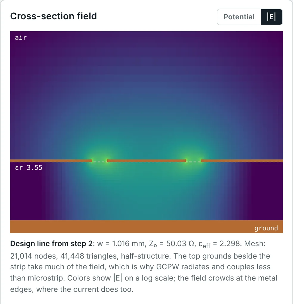
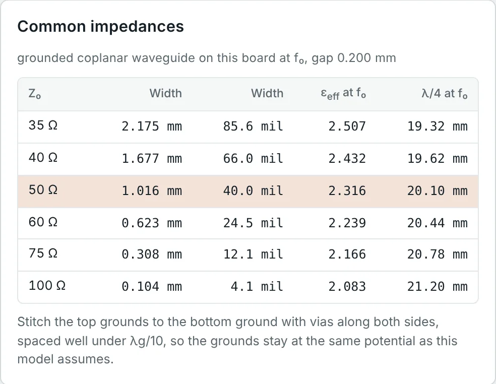
FEM electric field magnitude of a 50 ohm grounded coplanar waveguide on RO4003C with 0.2 mm gaps, concentrated in the slots — Fig 4a — |E| of a 1.016 mm, 50 Ω GCPW with 0.2 mm gaps on 0.813 mm RO4003C (35 µm copper). Try it in the Microstrip & Stripline Impedance Calculator →

Table of grounded CPW widths for 35 to 100 ohms with 0.2 mm gap on RO4003C at 2.45 GHz — Fig 4b — GCPW widths, εeff and λ/4 lengths at 2.45 GHz with 0.2 mm gaps. Try it in the Microstrip & Stripline Impedance Calculator →

The calculator's field solver also shows how strongly metal thickness matters in narrow-gap GCPW. With 35 µm copper and 0.2 mm gaps, the 50 Ω strip must be 1.016 mm wide; the zero-thickness closed form above predicts 1.178 mm — a 14% difference, because the copper edges facing each other across the slot add capacitance. For microstrip on the same board the difference was below 1%.

Gap s (RO4003C 0.813 mm)	50 Ω width, closed form (t = 0)	50 Ω width, FEM (t = 35 µm)	Overall w + 2s (FEM)
0.10 mm	0.832 mm	0.585 mm	0.785 mm
0.15 mm	—	0.840 mm	1.140 mm
0.20 mm	1.178 mm	1.016 mm	1.416 mm
0.30 mm	1.367 mm	1.243 mm	1.843 mm
0.50 mm	1.570 mm	1.475 mm	2.475 mm
1.00 mm	1.769 mm	1.672 mm	3.672 mm
∞ (microstrip)	1.819 mm	1.769 mm	—

CPW vs. Microstrip Transmission Lines

Property	CPW / GCPW	Microstrip
Impedance set by	w/s (and h for GCPW)	w/h
Size freedom	Any size for a given Z₀	Width fixed by h
Shunt grounding	Direct, no vias	Through vias
Dispersion	Lower	Higher
Radiation and coupling	Lower — field confined to slots	Higher
Conductor loss	Higher for the same width (edge crowding in narrow slots)	Lower
Sensitivity to etch tolerance	High for narrow gaps	Lower
Parasitic modes	Slot-line mode; parallel-plate mode in GCPW	Surface waves at high frequency
Typical use	MMICs, on-wafer probing, mm-wave PCBs, connector launches	General RF PCBs, patch antennas

Advantages and Limitations of CPW

AdvantagesShunt components without vias; easy probing; low dispersion and radiation; high isolation between adjacent lines (grounds between them); size freely scalable; natural transition to GSG probes, connectors and slot antennas.

LimitationsHigher conductor loss for small sizes; needs air bridges or vias to suppress the slot-line mode; more board area per line; impedance sensitive to narrow-gap etching and metal thickness; GCPW needs via fences against parallel-plate modes.

Practical CPW Design Calculations

The examples use the conformal-mapping formulas above, with K(k)/K(k′) from Hilberg's approximation, and c = 299.79 mm/ns.

Z₀ and εeff of CPW on Alumina

Problem: A CPW on 0.635 mm alumina (εr = 9.8) has w = 100 µm and s = 60 µm. Find Z₀ and εeff, first treating the substrate as thick, then with its actual height.

Thick-substrate formula (k = 100/220 = 0.4545 ≤ 0.707)

\frac{K (k)}{K (k^{'})} = \frac{π}{\ln [2 (1 + \sqrt{0.8907}) / (1 - \sqrt{0.8907})]} = \frac{π}{4.2365} = 0.7416

ε_{eff} = \frac{10.8}{2} = 5.40

Z_{0} = \frac{30 π}{\sqrt{5.4}} \times \frac{1}{0.7416} = 54.7 Ω

With h = 0.635 mm (Simons)

ε_{eff} = 5.377 Z_{0} = 54.8 Ω

Answer: Z₀ ≈ 54.7 Ω, εeff = 5.40 (thick); 54.8 Ω, εeff = 5.38 with h = 0.635 mm

The substrate is about three times thicker than w + 2s = 0.22 mm, so the thick-substrate formula is accurate to 0.2%. For 50 Ω the gaps must close to about 44 µm.

Choosing the Gap for 50 Ω

Problem: Keeping w = 100 µm on alumina, find the gap that gives 50 Ω. What k does it correspond to?

Required K(k′)/K(k) for 50 Ω (εeff = 5.38)

\frac{K (k^{'})}{K (k)} = \frac{50 \sqrt{5.38}}{30 π} = 1.231

\Rightarrow k \approx 0.532 \Rightarrow s = \frac{w (1 - k)}{2 k} = 44 μ m

Answer: s ≈ 44 µm (k ≈ 0.53)

Any line with k = 0.53 is 50 Ω on alumina: 50 µm with 22 µm gaps for a compact MMIC-style layout, or 200 µm with 88 µm gaps for lower loss. Thin-film alumina processes etch such gaps routinely.

A 50 Ω CPW on a GaAs MMIC

Problem: On a 100 µm GaAs MMIC (εr = 12.9) with a 50 µm centre strip, find the gap for 50 Ω. How wrong would the thick-substrate formula be?

Simons' formula with h = 100 µm, solved for Z₀ = 50 Ω

s = 31.6 μ m k = \frac{50}{113.1} = 0.442 ε_{eff} = 6.65

Thick-substrate formula with the same dimensions

ε_{eff} = 6.95 Z_{0} = 48.9 Ω

Answer: s ≈ 32 µm; the thick-substrate formula would be 1.1 Ω (2%) low

Here h is only 0.9 × (w + 2s), so the finite thickness lowers εeff by 4%. On thin MMIC substrates the full formula — or an EM solver — is needed.

What the Bottom Ground Does

Problem: A line with w = 1.0 mm and s = 0.2 mm is etched on 0.813 mm RO4003C. Compare Z₀ and εeff with and without a ground plane on the back (zero-thickness closed forms).

Without a back ground (CPW, Simons)

Z_{0} = 63.9 Ω ε_{eff} = 2.14

With a back ground (GCPW)

Z_{0} = 53.7 Ω ε_{eff} = 2.41

Answer: adding the bottom ground lowers Z₀ by 10 Ω and raises εeff from 2.14 to 2.41

The bottom ground adds capacitance and pulls more field into the substrate. A CPW on a PCB must therefore be designed knowing what lies below it — a bottom copper layer, a metal enclosure floor or air.

Why the Field Solver Disagrees with the Closed Form

Problem: For 50 Ω GCPW with 0.2 mm gaps on 0.813 mm RO4003C, the closed form gives w = 1.178 mm and the FEM solver (35 µm copper) gives w = 1.016 mm. Explain the difference and estimate the extra capacitance.

Side-wall capacitance of the two slot edges (parallel-plate estimate, per metre)

Δ C \approx 2 \times ε_{0} \frac{t}{s} = 2 \times 8.854 pF/m \times \frac{0.035}{0.2} = 3.1 pF/m

Answer: thick copper adds capacitance across the slots and lowers Z₀ by about 3.4 Ω, so the strip must be narrower

The line capacitance of a 50 Ω GCPW with εeff ≈ 2.3 is √εeff/(cZ₀) ≈ 101 pF/m. The side walls alone add about 3 pF/m directly, and the thick edges add further fringing capacitance; at the closed-form width the 35 µm copper lowers Z₀ from 53.4 Ω (t = 0, w = 1.016 mm) to 50.0 Ω. Because Z₀ changes only slowly with w in narrow-gap GCPW, compensating this needs a 14% narrower strip. In microstrip the same copper changed the width by only 1%. Always use a thickness-aware calculator for narrow-gap GCPW.

Sizing a GCPW to Match 0402 Component Pads

Problem: A filter uses 0402 components with 0.5–0.6 mm wide pads on 0.813 mm RO4003C with 35 µm copper. Choose a 50 Ω GCPW whose strip matches the pads.

From the FEM gap sweep (table above)

s = 0.10 mm \Rightarrow w = 0.585 mm

(microstrip would need w = 1.769 mm)

Answer: w = 0.585 mm with 0.10 mm gaps

The pads now sit on the line with no width step, eliminating the step discontinuity a 1.77 mm microstrip would need (Part 13). The 0.1 mm gap is at the limit of standard PCB etching, so the impedance tolerance must be checked with the fabricator.

Via-Fence Spacing for a 24 GHz GCPW

Problem: A 50 Ω GCPW on RO4003C has εeff ≈ 2.32. Find λ_g at 24 GHz and the maximum via spacing by the λ_g/10 rule (λ_g/20 for a conservative design).

Guided wavelength and spacing

λ_{g} = \frac{299.79}{24 \sqrt{2.32}} = 8.20 mm

\frac{λ_{g}}{10} = 0.82 mm

\frac{λ_{g}}{20} = 0.41 mm

Answer: via pitch ≤ 0.8 mm, preferably about 0.4–0.5 mm

The vias should also sit close to the slot edges (within about s to 2s) so that the top grounds are tied down where the return current flows. Part 11 develops the via-fence design rules.

Air-Bridge Spacing on an MMIC

Problem: On the GaAs CPW of Example 3 (εeff = 6.65), air bridges must be closer than λ_g/8 at the highest operating frequency of 40 GHz. What spacing is required?

Guided wavelength at 40 GHz

λ_{g} = \frac{299.79}{40 \sqrt{6.65}} = 2.91 mm \frac{λ_{g}}{8} = 0.36 mm

Answer: air bridges no more than about 0.36 mm apart — and at every bend, T-junction and discontinuity

Each air bridge adds a little capacitance to the centre strip, so long lines use as few as possible and compensate their effect in the design; at discontinuities, where the slot-line mode is generated, they are mandatory.

The Parallel-Plate Resonance of Unstitched GCPW

Problem: A GCPW board on RO4003C (εr = 3.55) has top-ground areas 30 mm long with no vias to the bottom ground. At what frequency does the first parallel-plate resonance between top and bottom grounds occur?

Half-wave resonance of a parallel-plate region of length L

f_{1} = \frac{c}{2 L \sqrt{ε_{r}}} = \frac{299.79}{2 \times 30 \times 1.884} = 2.65 GHz

Answer: about 2.65 GHz — well inside the band of most RF boards

At this frequency the ground region rings like a patch antenna, couples to the line and produces a sharp notch in S₂₁. Stitching vias every few millimetres push the resonance far above the band; that is their main purpose.

Loss of GCPW Compared with Microstrip

Problem: On 0.813 mm RO4003C at 2.45 GHz the calculator gives 0.0197 dB/cm for 50 Ω microstrip and 0.0291 dB/cm for the 50 Ω GCPW with 0.2 mm gaps (74% of it conductor loss). Why is GCPW lossier, and by how much over a 100 mm line?

Loss over 100 mm

microstrip : 0.197 dB GCPW : 0.291 dB

Answer: GCPW loses about 0.1 dB more per 100 mm, because its 1.0 mm strip (versus 1.77 mm) and narrow gaps concentrate the current

For the same impedance, GCPW with narrow gaps has a narrower strip and strong current crowding at the slot edges, so its conductor loss is higher. Widening the gaps reduces the loss towards the microstrip value; GCPW is chosen for its isolation, grounding and transitions, not for the lowest loss.

Summary

CPW: a centre strip between two coplanar grounds; it supports the wanted CPW mode and an unwanted slot-line mode, suppressed by air bridges or vias.
Conformal mapping gives exact quasi-static results: Z₀ = (30π/√εeff) K(k′)/K(k), k = w/(w + 2s), and εeff = (εr + 1)/2 on a thick substrate.
Z₀ depends on w/s, not on absolute size; thin substrates (h < w + 2s) lower εeff and raise Z₀.
Grounded CPW adds a back ground: a microstrip–CPW hybrid that needs via fences to suppress parallel-plate modes.
Metal thickness matters much more than in microstrip for narrow gaps — use a thickness-aware solver.
CPW offers easy grounding, low dispersion and radiation and free sizing; it pays with higher conductor loss and parasitic-mode control.

CPW keeps its grounds on the surface; stripline buries the signal between two grounds. Part 11: Stripline and Grounded Coplanar Waveguide covers symmetric and asymmetric stripline, then returns to grounded CPW with via fences, and compares the three planar lines for multilayer RF boards.

📘 Go deeper: Matching with CPW

Stubs and quarter-wave transformers in CPW are designed on the Smith chart exactly as in microstrip. Open Smith Chart & Impedance Matching series →

Put It Into Practice

Use the NEXT ANTENNAS calculators to apply the ideas from this article to real lines and circuits.

Transmission Lines Microstrip & Stripline Impedance Calculator Field-solver backed design of microstrip, embedded microstrip, stripline, GCPW and differential pairs: width, εeff, Z₀, loss, dispersion and tolerance. Open calculator → Impedance Matching Smith Chart Visualiser Plot impedances, move along lines and stubs, load Touchstone files and design matching networks. Open calculator → Antenna & Signal Wavelength / Frequency Calculator Convert between frequency and wavelength in free space and in dielectrics. Open calculator → All Tools All RF Calculators Browse every NEXT ANTENNAS calculator for RF, microwave and antenna design. Open calculator →

Coplanar Waveguide (CPW)