Coplanar waveguide — structure & field distribution

A CPW places the signal conductor and both ground planes on the same surface of the substrate. The signal conductor of width w is flanked by two symmetric slots of width g, beyond which lie the ground planes. The substrate has thickness h and relative permittivity ε_r. The field is confined primarily in the two slots, allowing surface-mount probing without vias.

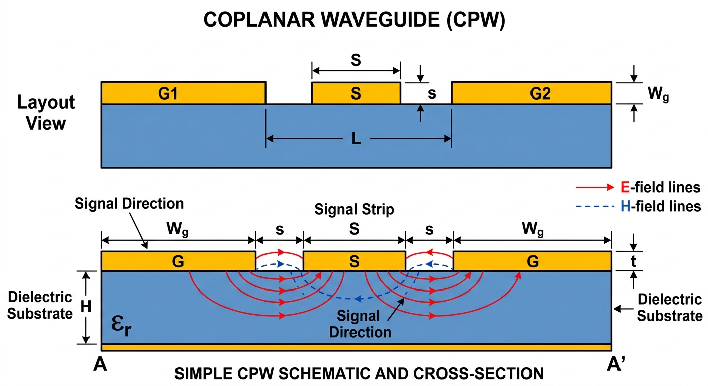
Coplanar waveguide CPW cross-section showing signal conductor, slot gaps, ground planes, dielectric substrate, and electric and magnetic field distributions

k = w/(w+2g) = 0.600 Quasi-TEM Mode Coplanar Line

Center Trace Width (w) 1.50 mm

Slot Gap Spacing (g) 0.50 mm

Substrate

Relative permittivity εr

Substrate thickness h (mm)

Conductor thickness t (mm)

Common substrates

Editing εr / h / t clears the preset selection.

CPW geometry

Signal conductor width w (mm)

Slot gap width g (mm)

Target Z₀ presets

Frequency f (GHz)

Results

Signal width w

—

Slot gap g

—

Fill ratio k = w/(w+2g)

—

dimensionless

Characteristic Z₀

—

Effective εeff

—

εeff

Phase velocity

—

×10⁸ m/s

Guided wavelength

λg (full wave)

—

λg / 2

—

λg / 4

—

Additional outputs

Wave number β

—

rad/m

Free-space λ₀

—

mm at freq

Slowdown factor

—

vp / c

Frequency GHz

λg = vp / f = (c / √εeff) / f · β = 2π / λg

⚠ Geometry outside typical range — verify with EM simulation.

Method & reference

Uses conformal mapping with complete elliptic integrals K(k) computed via the arithmetic-geometric mean (AGM) algorithm — equivalent to full numerical integration, converging in under 20 iterations. The finite-substrate correction is applied through a modified fill ratio using hyperbolic functions of w, g, and h. Conductor thickness correction follows Schneider's approximation when t > 0. Valid for h ≫ g and w/h > 0.1.

Reference: Ghione & Naldi, IEEE Trans. MTT, 1987. Also: Simons, Coplanar Waveguide Circuits, Components, and Systems, Wiley 2001.

📐 Design your antenna Patch Antenna Calculator Compute patch width, length, inset feed depth, and notch gap for any substrate and frequency. → 〰️ Compare transmission lines Microstrip Width Calculator Compute microstrip trace width, εeff, phase velocity, and guided wavelength using Hammerstad–Jensen synthesis. →

What Is a Coplanar Waveguide?

A coplanar waveguide (CPW) is a planar transmission line in which the signal conductor and both return ground planes lie on the same surface of the substrate. Invented by C. P. Wen in 1969, CPW is now the dominant transmission line format for MMICs, millimetre-wave probes, and high-speed PCB interconnects because the ground reference is always accessible from the top surface without requiring via holes through the substrate.

Key advantages over microstrip

Same-layer ground access — shunt components connect to ground without vias, eliminating parasitic via inductance
Ground-signal-ground (GSG) probing — on-wafer and on-board RF probes land directly on the CPW pattern
Impedance set by the w/g ratio — independent of substrate thickness, enabling compact designs on any dielectric
Lower dispersion at mm-wave — field confined in the slots rather than the full substrate thickness
Flip-chip and wire-bond compatible — all interconnects on a single surface layer

Design Variables

Symbol	Name	Typical range
w	Signal conductor width	0.1 – 5 mm
g	Slot gap width	0.05 – 2 mm
h	Substrate thickness	0.127 – 3.175 mm
εr	Relative permittivity	2.1 – 12
t	Conductor thickness	5 μm – 70 μm
k	Fill ratio w / (w + 2g)	0 – 1 (dimensionless)

Characteristic Impedance — Conformal Mapping

The CPW cross-section is mapped conformally to a parallel-plate capacitor via the Schwarz–Christoffel transformation. The result expresses Z₀ as a ratio of complete elliptic integrals of the first kind K(k).

Fill ratio k (infinite substrate)

k = w w + 2g , k' = √(1 − k²)

w = signal conductor width · g = slot gap · k → 1 means very wide conductor (low Z₀) · k → 0 means narrow conductor (high Z₀)

Finite substrate correction — fill ratio k₁

k₁ = sinh(πw / 4h) sinh(π(w + 2g) / 4h) , k₁' = √(1 − k₁²)

h = substrate thickness · as h → ∞, k₁ → k (recovers the infinite-substrate case)

Effective permittivity εeff

εeff = 1 + εr − 1 2 · K(k₁') · K(k) K(k₁) · K(k')

K(k) = complete elliptic integral of the first kind · the substrate filling factor weights εr against unity

Characteristic impedance Z₀

Z₀ = 30π √εeff · K(k') K(k)

For 50 Ω on FR-4 (εr = 4.4, h = 1.6 mm): typical starting point is w = 1.5 mm, g = 0.5 mm

Elliptic Integral — AGM Algorithm

K(k) has no closed-form expression but converges rapidly using the arithmetic-geometric mean (AGM):

AGM algorithm for K(k)

a₀ = 1, b₀ = k' = √(1 − k²)

aₙ₊₁ = aₙ + bₙ2 , bₙ₊₁ = √(aₙ · bₙ)

K(k) = π2 · a∞ (a∞ = AGM limit, converges in ~15 iterations)

CPW vs Microstrip

Property	CPW	Microstrip
Ground reference layer	Same surface as signal	Opposite surface
Via holes for shunt elements	Not required	Required
GSG RF probe landing	Direct	Requires adaptation
Impedance control parameter	w/g ratio	w/h ratio
Substrate thickness dependence	Weak (finite h correction only)	Strong
mm-wave dispersion	Lower	Higher
Radiation / leakage at low freq	Higher	Lower

50 Ω starting point on FR-4 (εr = 4.4, h = 1.6 mm): Set signal width w = 1.5 mm and slot gap g = 0.5 mm. The fill ratio k = w/(w+2g) = 0.60 yields Z₀ ≈ 50 Ω. To increase Z₀, widen the slots (larger g) or narrow the signal conductor (smaller w). To decrease Z₀, do the opposite. The ground plane extent beyond each slot should be at least 5× the slot gap to approximate an infinite ground plane.

If your design uses microstrip rather than CPW — or if you need to transition between the two on the same board — use our Microstrip Width Calculator to compute the equivalent 50 Ω trace width, effective permittivity, and guided wavelength for your substrate. Both tools use the same substrate presets, so you can compare results side by side.

〰️ Single-sided ground plane alternative Microstrip Width Calculator Hammerstad–Jensen synthesis for trace width W, εeff, phase velocity, and guided wavelength — same substrates, instant results. →

Coplanar Waveguide (CPW) Calculator